Book 2.indb - US Climate Change Science Program

TABLE OF CONTENTSAuthor Team for this Report..............................................................................IVAcknowledgments.................................................................................................VRecommended Citations....................................................................................VISynopsis............................................................................................................... VIIPreface................................................................................................................ VIIIExecutive Summary...............................................................................................1CHAPTER1..............................................................................................................................9Introduction: Abrupt Changes in the Earth’s Climate System2............................................................................................................................29Rapid Changes in Glaciers and Ice Sheets and their Impacts on Sea Level3............................................................................................................................67Hydrological Variability and Change4.......................................................................................................................... 117The Potential for Abrupt Change in the Atlantic Meridional OverturningCirculation5..........................................................................................................................163Potential for Abrupt Changes in Atmospheric MethaneReferences.......................................................................................................... 202Photography Credits.........................................................................................239Glossary, Acronyms, and Abbreviations.........................................................241III

IIAUTHOR TEAM FOR THIS REPORTPrefaceLead Authors: John P. McGeehin, USGS; John A. Barron, USGS; David M. Anderson,NOAA; David J. Verardo, NSFExecutive SummaryLead Authors: Peter U. Clark, Oregon State University; Andrew J. Weaver,University of VictoriaContributing Authors: Edward Brook, Oregon State University; Edward R. Cook,Columbia University; Thomas L. Delworth, NOAA; Konrad Steffen,University of ColoradoChapter 1Lead Authors: Peter U. Clark, Oregon State University; Andrew J. Weaver,University of VictoriaContributing Authors: Edward Brook, Oregon State University; Edward R. Cook,Columbia University; Thomas L. Delworth, NOAA; Konrad Steffen,University of ColoradoChapter 2Lead Author: Konrad Steffen, University of ColoradoContributing Authors: Peter U. Clark, Oregon State University; J. Graham Cogley,Trent University; David Holland, New York University; Shawn Marshall,University of Calgary; Eric Rignot, University of California, NASA JPL, andCentro de Estudios Cientificos, Valdivia, Chile; Robert Thomas, EG&G Services,NASA Goddard Space Flight Center, Wallops Flight Facility, and Centro de EstudiosCientificos, Valdivia, ChileChapter 3Lead Author: Edward R. Cook, Columbia UniversityContributing Authors: Patrick J. Bartlein, University of Oregon; Noah Diffenbaugh,Purdue University; Richard Seager, Columbia University; Bryan N. Shuman,University of Wyoming; Robert S. Webb, NOAA; John W. Williams,University of Wisconsin; Connie Woodhouse, University of ArizonaChapter 4Lead Author: Thomas L. Delworth, NOAAContributing Authors: Peter U. Clark, Oregon State University; Marika Holland,National Center for Atmospheric Research; William E. Johns, University of Miami;Till Kuhlbrodt, University of Reading; Jean Lynch-Stieglitz, Georgia Instituteof Technology; Carrie Morrill, University of Colorado/NOAA; Richard Seager,Columbia University; Andrew J. Weaver, University of Victoria; Rong Zhang, NOAAChapter 5Lead Author: Edward Brook, Oregon State UniversityContributing Authors: David Archer, University of Chicago; Ed Dlugokencky, NOAA;Steve Frolking, University of New Hampshire; David Lawrence, National Centerfor Atmospheric ResearchIV

The U.S. Climate Change Science ProgramPrefaceRECOMMENDED CITATIONSFor the Report as a whole:CCSP, 2008: Abrupt Climate Change. A report by the U.S. Climate Change Science Program and the Subcommittee onGlobal Change Research [Clark, P.U., A.J. Weaver (coordinating lead authors), E. Brook, E.R. Cook, T.L. Delworth,and K. Steffen (chapter lead authors)]. U.S. Geological Survey, Reston, VA, 244 pp.For the Preface:McGeehin, J.P., J.A. Barron, D.M. Anderson, and D.J. Verardo, 2008: Preface. In: Abrupt Climate Change. A report bythe U.S. Climate Change Science Program and the Subcommittee on Global Change Research. U.S. Geological Survey,Reston, VA, pp. VIII–X.For the Executive Summary:Clark, P.U., A.J. Weaver, E. Brook, E.R. Cook, T.L. Delworth, and K. Steffen, 2008: Executive Summary. In: AbruptClimate Change. A Report by the U.S. Climate Change Science Program and the Subcommittee on Global ChangeResearch. U.S. Geological Survey, Reston, VA, pp. 1–7.For Chapter 1:Clark, P.U., A.J. Weaver, E. Brook, E.R. Cook, T.L. Delworth, and K. Steffen, 2008: Introduction: Abrupt changes in theEarth's climate system. In: Abrupt Climate Change. A Report by the U.S. Climate Change Science Program and theSubcommittee on Global Change Research. U.S. Geological Survey, Reston, VA, pp. 9–27.For Chapter 2:Steffen, K., P.U. Clark, J.G. Cogley, D. Holland, S. Marshall, E. Rignot, and R. Thomas, 2008: Rapid changes in glaciersand ice sheets and their impacts on sea level. In: Abrupt Climate Change. A Report by the U.S. Climate Change ScienceProgram and the Subcommittee on Global Change Research. U.S. Geological Survey, Reston, VA, pp. 29–66.For Chapter 3:Cook, E.R., P.J. Bartlein, N. Diffenbaugh, R. Seager, B.N. Shuman, R.S. Webb, J.W. Williams, and C. Woodhouse, 2008:Hydrological variability and change. In: Abrupt Climate Change. A Report by the U.S. Climate Change Science Programand the Subcommittee on Global Change Research. U.S. Geological Survey, Reston, VA, pp. 67–115.For Chapter 4:Delworth, T.L., P.U. Clark, M. Holland, W.E. Johns, T. Kuhlbrodt, J. Lynch-Stieglitz, C. Morrill, R. Seager, A.J. Weaver,and R. Zhang, 2008: The potential for abrupt change in the Atlantic Meridional Overturning Circulation. In: AbruptClimate Change. A report by the U.S. Climate Change Science Program and the Subcommittee on Global Change Research.U.S. Geological Survey, Reston, VA, pp. 117–162.For Chapter 5:Brook, E., D. Archer, E. Dlugokencky, S. Frolking, and D. Lawrence, 2008: Potential for abrupt changes in atmosphericmethane. In: Abrupt Climate Change. A report by the U.S. Climate Change Science Program and the Subcommittee onGlobal Change Research. U.S. Geological Survey, Reston, VA, pp. 163–201.VI

Weather and Climate Extremes in a Changing ClimateRegions of focus: North America, Hawaii, Caribbean, and U.S. Pacific IslandsSYNOPSISFor this Synthesis and Assessment Report, abrupt climate change is defined as:A large-scale change in the climate system that takes place overa few decades or less, persists (or is anticipated to persist) for atleast a few decades, and causes substantial disruptions in humanand natural systems.This report considers progress in understanding four types of abrupt changein the paleoclimatic record that stand out as being so rapid and large in theirimpact that if they were to recur, they would pose clear risks to society in termsof our ability to adapt: (1) rapid change in glaciers, ice sheets, and hence sealevel; (2) widespread and sustained changes to the hydrologic cycle; (3) abruptchange in the northward flow of warm, salty water in the upper layers of theAtlantic Ocean associated with the Atlantic Meridional Overturning Circulation(AMOC); and (4) rapid release to the atmosphere of methane trapped inpermafrost and on continental margins.This report reflects the significant progress in understanding abrupt climatechange that has been made since the report by the National Research Councilin 2002 on this topic, and this report provides considerably greater detail andinsight on these issues than did the 2007 Intergovernmental Panel on ClimateChange Fourth Assessment Report (IPCC AR4). New paleoclimatic reconstructionshave been developed that provide greater understanding of patternsand mechanisms of past abrupt climate change in the ocean and on land, andnew observations are further revealing unanticipated rapid dynamic changesof modern glaciers, ice sheets, and ice shelves as well as processes that arecontributing to these changes. This report reviews this progress. A summaryand explanation of the main results is presented first, followed by an overviewof the types of abrupt climate change considered in this report. The subsequentchapters then address each of these types of abrupt climate change, including asynthesis of the current state of knowledge and an assessment of the likelihoodthat one of these abrupt changes may occur in response to human influenceson the climate system.IIVII

PREFACEReport Motivation and Guidance for Using thisSynthesis and Assessment ReportLead Authors:John P. McGeehin, USGSJohn A. Barron, USGSDavid M. Anderson, NOAADavid J. Verardo, NSFA primary objective of the U.S. Climate Change ScienceProgram (CCSP) is to provide the best possible,up-to-date scientific information to support publicdiscussion and government and private sector decisionmakingon key climate-related issues. To help meet thisobjective, the CCSP has identified a set of 21 synthesisand assessment products (SAP) to address its highestpriority research, observation, and decision-supportneeds. This SAP (3.4) focuses on abrupt climate changeevents where key aspects of the climate system changefaster than the responsible forcings would suggest and/or faster than society can respond to those changes.This report addresses Goal 3 of the CCSP StrategicPlan: Reduce uncertainty in projections of how theEarth’s climate and related systems may change inthe future. The report (1) summarizes the currentknowledge of key climate parameters that could changeabruptly in the near future, potentially within years todecades and (2) provides scientific information on thesetopics for decision support. As such, the SAP is aimedat both the decision-making audience and the expertscientific and stakeholder community.BackgroundPast records of climate and environmental change derivedfrom archives such as tree rings, ice cores, corals,and sediments indicate that global and regional climatehas experienced repeated abrupt changes, many occurringover a time span of decades or less. Abrupt climatechanges might have a natural cause (such as volcanicaerosol forcing), an anthropogenic cause (such as increasingcarbon dioxide in the atmosphere), or mightbe unforced (related to internal climate variability).Regardless of the cause, abrupt climate change presentspotential risks for society that are poorly understood.An improved ability to understand and model futureabrupt climate change is essential to provide decisionmakerswith the information they need to plan for thesepotentially significant changes.The National Research Council (NRC) report“Abrupt Climate Change” (Alley et al., 2002)provides an excellent treatise on this topic. Additionally,the Intergovernmental Panel on ClimateChange Fourth Assessment Report (IPCC AR4)(IPCC, 2007) addresses many of the same topicsassociated with abrupt climate change. This SAPpicks up where the NRC report and the IPCC AR4leave off, updating the state and strength of existingknowledge, both from the paleoclimate and historicalrecords, as well as from model predictions forfuture change.Focus of this Synthesis and AssessmentProductThe content of this report follows a prospectus thatwas developed by the SAP Product Advisory Group,made up of the co-authors of this preface. The prospectusis available from the CCSP website (http://www.climatescience.gov).SAP 3.4 considers four types of change documentedin the paleoclimate record that stand out as being sorapid and large in their impact that they pose clearrisks to society in terms of our ability to adapt.They are supported by sufficient evidence in currentresearch indicating that abrupt changes could occurin the future. These four topics, each addressed as achapter in this report, are1. Rapid Changes in Glaciers and Ice Sheetsand their Impacts on Sea Level;2. Hydrological Variability and Change;3. Potential for Abrupt Change in theAtlantic Meridional OverturningCirculation (AMOC); and4. Potential for Abrupt Changes inAtmospheric Methane.VIII

Abrupt Climate ChangeThe following questions are considered in this report:Rapid Changes in Glaciers and Ice Sheets and theirImpacts on Sea Level• What is the paleoclimate evidence regarding ratesof rapid ice sheet melting?• What are the recent rates and trends in ice sheetmass balance?• What will be the impact on sea level if the recentlyobserved rapid rates of melting continue?• What is needed to model the mechanical processesthat accelerate ice loss?Hydrological Variability and Change• What is our present understanding of the causes ofmajor drought and hydrological change, including therole of the oceans or other natural or nongreenhousegasanthropogenic effects as well as land-use changes?(Note that this question is posed to facilitate an assessmentof what is known about natural causes forhydrological change as opposed to anthropogeniccauses, such as increased greenhouse gases. Theauthors also address anthropogenic influences, includinggreenhouse gases, as a potential source ofhydrological change, in the past, present, and future.)• What is our present understanding of the duration,extent, and causes of megadroughts of the past2,000 years?• What states of oceanic/atmospheric conditions andthe strength of land-atmosphere coupling are likely tohave been responsible for sustained megadroughts?• How might such a state affect the climate in regionsnot affected by drought? (For example, enhancedfloods or hurricanes in other regions.)• What will be the change in the state of natural variabilityof the ocean and atmosphere that will signalthe abrupt transition to a megadrought?Potential for Abrupt Change in the Atlantic MeridionalOverturning Circulation• What are the factors that control the overturningcirculation?• How well do the current ocean general circulationmodels (and coupled atmosphere-ocean models)simulate the overturning circulation?• What is the present state of the MOC?• What is the evidence for change in the overturningcirculation in the past?• What are the global and regional impacts of achange in the overturning circulation?• What factors that influence the overturning circulationare likely to change in the future, and what is theprobability that the overturning circulation will change?• What are the observational and modeling requirementsrequired to understand the overturning circulationand evaluate future change?Potential for Abrupt Changes in Atmospheric Methane• What is the volume of methane stored in terrestrialand marine sources and how much of it is likely to bereleased in various climate change scenarios?• What is the impact on the climate system of therelease of varying quantities of methane over varyingintervals of time?• What is the evidence in the past for abrupt climatechange caused by massive methane release?• How much methane is likely to be released bythawing of the topmost layer (3 meters) of permafrost?Is thawing at greater depths likely to occur?• What conditions (in terms of sea-level rise andwarming of bottom waters) would allow methanerelease from hydrates in sea-floor sediments?• What are the observational and modeling requirementsnecessary to understand methane storage andits release under various future scenarios of abruptclimate change?Each section of this report is structured to answer thesequestions in the manner that best suits the topic. Questionsare addressed either specifically as individual sections orsubsections of a chapter, or through a broader, more systematicdiscussion of the topic. Additional subject matteris presented in a chapter, beyond what is asked for in theprospectus, where the authors feel that this information isnecessary to effectively treat the topic.It is important to note that the CCSP Synthesis and AssessmentProducts are scientific documents that are intended tobe of use not only to scientists but to the American publicand to decisionmakers within the United States. As such,the geographic focus of the Abrupt Climate Change SAP isUnited States, and by extension, North American climate.Other regional examples of abrupt climate change are discussedwhen the authors feel that the information servesas an important analog to past, present, or future NorthAmerican climate.Suggestions for Reading, Using, andNavigating this ReportThis report is composed of four main chapters that correspondto the major climate themes indicated above. Thereis also an introductory chapter that provides an extensiveoverview of the information from the other four chapters, aswell as additional background information. The ExecutiveSummary further distills the information, with a focus onthe key findings and recommendations from each chapter.IX 11

The U.S. Climate Change Science ProgramThe four theme chapters have a recurring organizationalformat. Each chapter begins with key scientific findingswhich are then followed by recommendations for futureresearch aimed at deepening our understanding of thecritical scientific issues raised in the chapter. The scientifictheories, models, data, and uncertainties that are part of theauthor’s scientific syntheses and assessments are referencedthrough citations to peer-reviewed literature throughout thechapter. Finally, side boxes are used to discuss topics theauthor team felt deserved additional attention or served asuseful case studies.A reader interested in an overview of the state of the sciencefor the topic of abrupt climate change might, therefore, startby reading the Executive Summary and Introduction chapter(Chapter 1) of this report, then delve deeper into the thematicchapters for more detailed explanations and information.To integrate a wide variety of information and provideestimates of uncertainty associated with results, this reportutilizes the terms from the IPCC AR4 (IPCC, 2007).Terms of uncertainty range from “exceptionally unlikely”(< 1% likelihood) to “virtually certain” (> 99% likelihood).See Box 1.1 in the Introduction chapter (Chapter 1) of thisreport for a complete explanation of the uncertainty terms.The Synthesis and Assessment Product TeamThe primary authors of this report were constituted as aFederal Advisory Committee that was charged with advisingthe USGS and the CCSP on the scientific and technicalcontent related to the topic of abrupt climate change as describedin the SAP 3.4 prospectus. (See Public Law 92-463for more information on the Federal Advisory CommitteeAct, and the GSA website http://fido.gov/facadatabase/ forspecific information related to the SAP 3.4 Federal AdvisoryCommittee.) The Federal Advisory Committee for SAP 3.4enlisted input from numerous contributing authors. Theseauthors provided substantial, relevant content to the report,but did not participate in the Federal Advisory Committeedeliberations upon which this SAP was developed.ReferencesAlley, R.B., et al., 2002: Abrupt climate change: Inevitablesurprises. National Academy Press, Washington, DC,244 pp.IPCC, 2007: Climate change 2007. The physical sciencebasis. Contribution of Working Group I to the FourthAssessment Report of the Intergovernmental Panel onClimate Change [Solomon, S., D. Qin, M. Manning, Z.Chen, M. Marquis, K.B. Averyt, M. Tignor, and H.L.Miller (eds.)]. Cambridge University Press, Cambridge,United Kingdom, 996 pp.PrefaceX

Abrupt Climate ChangeEXECUTIVE SUMMARYLead Authors: Peter U. Clark,* Department of Geosciences,Oregon State UniversityAndrew j. Weaver,* School of Earth and Ocean Sciences,University of Victoria, CanadaContributing Authors: Edward Brook,* Department ofGeosciences, Oregon State UniversityEdward R. Cook,* Lamont-Doherty Earth Observatory,Columbia UniversityThomas L. Delworth,* NOAA Geophysical Fluid DynamicsLaboratorykonrad Steffen,* Cooperative Institute for Research inEnvironmental Sciences, University of Colorado* SAP 3.4 Federal Advisory Committee memberMAIN RESULTS AND FINDINGSFor this Synthesis and Assessment Report,abrupt climate change is defined as:A large-scale change in the climatesystem that takes place over a fewdecades or less, persists (or is anticipatedto persist) for at least a few decades,and causes substantial disruptions inhuman and natural systems.This report considers progress in understandingfour types of abrupt change in the paleoclimaticrecord that stand out as being so rapid and largein their impact that if they were to recur, theywould pose clear risks to society in terms ofour ability to adapt: (1) rapid change in glaciers,ice sheets, and hence sea level; (2) widespreadand sustained changes to the hydrologic cycle;(3) abrupt change in the northward flow ofwarm, salty water in the upper layers of theAtlantic Ocean associated with the AtlanticMeridional Overturning Circulation (AMOC);and (4) rapid release to the atmosphere of methanetrapped in permafrost and on continentalmargins. While these four types of changepose clear risks to human and natural systems,this report does not focus on specific effectson these systems as a result of abrupt change.This report reflects the significant progress inunderstanding abrupt climate change that hasbeen made since the report by the NationalResearch Council in 2002 on this topic, andthis report provides considerably greater detailand insight on these issues than did the 2007Intergovernmental Panel on Climate Change(IPCC) Fourth Assessment Report (AR4).New paleoclimatic reconstructions have beendeveloped that provide greater understandingof patterns and mechanisms of past abrupt climatechange in the ocean and on land, and newobservations are further revealing unanticipatedrapid dynamic changes of modern glaciers, icesheets, and ice shelves as well as processes thatare contributing to these changes. This reportreviews this progress. A summary and explanationof the main results is presented first,followed by an overview of the types of abruptclimate change considered in this report. Thesubsequent chapters then address each of thesetypes of abrupt climate change, including asynthesis of the current state of knowledge andan assessment of the likelihood that one of theseabrupt changes may occur in response to humaninfluences on the climate system. Throughoutthis report we have adopted the IPCC terminologyin our expert assessment of the likelihoodof a particular outcome or result. The termvirtually certain implies a >99% probability;extremely likely: >95% probability; very likely:>90% probability; likely: >66% probability;more likely than not: >50% probability; aboutas likely as not: 33%–66% probability; unlikely:

The U.S. Climate Change Science ProgramBased on an assessment of the publishedscientific literature, the primary conclusionspresented in this report are:• Recent rapid changes at the edges of theGreenland and West Antarctic ice sheetsshow acceleration of flow and thinning,with the velocity of some glaciers increasingmore than twofold. Glacier accelerationscausing this imbalance have beenrelated to enhanced surface meltwater productionpenetrating to the bed to lubricateglacier motion, and to ice-shelf removal,ice-front retreat, and glacier ungroundingthat reduce resistance to flow. The presentgeneration of models does not capture theseprocesses. It is unclear whether this imbalanceis a short-term natural adjustment ora response to recent climate change, butprocesses causing accelerations are enabledby warming, so these adjustments will verylikely become more frequent in a warmerclimate. The regions likely to experiencefuture rapid changes in ice volume arethose where ice is grounded well below sealevel such as the West Antarctic Ice Sheetor large glaciers in Greenland like the JakobshavnIsbræ that flow into the sea througha deep channel reaching far inland. Inclusionof these processes in models will likelylead to sea-level projections for the end ofthe 21st century that substantially exceedthe projections presented in the IPCC AR4report (0.28 ± 0.10 m to 0.42 ± 0.16 m rise).• There is no clear evidence to date ofhuman-induced global climate change onNorth American precipitation amounts.However, since the IPCC AR4 report,further analysis of climate model scenariosof future hydroclimatic change over NorthAmerica and the global subtropics indicatesthat subtropical aridity is likely tointensify and persist due to future greenhousewarming. This projected dryingextends poleward into the United StatesSouthwest, potentially increasing the likelihoodof severe and persistent droughtthere in the future. If the model results arecorrect, then this drying may have alreadybegun, but currently cannot be definitivelyidentified amidst the considerable naturalvariability of hydroclimate in SouthwesternNorth America.Executive Summary• The AMOC is the northward flow ofwarm, salty water in the upper layers ofthe Atlantic, and the southward flow ofcolder water in the deep Atlantic. It playsan important role in the oceanic transportof heat from low to high latitudes. It is verylikely that the strength of the AMOC willdecrease over the course of the 21st centuryin response to increasing greenhouse gases,with a best estimate decrease of 25–30%.However, it is very unlikely that the AMOCwill undergo an abrupt transition to a weakenedstate or collapse during the course ofthe 21st century, and it is unlikely that theAMOC will collapse beyond the end of the21st century because of global warming,although the possibility cannot be entirelyexcluded.• A dramatic abrupt release of methane (CH 4 )to the atmosphere appears very unlikely,but it is very likely that climate change willaccelerate the pace of persistent emissionsfrom both hydrate sources and wetlands.Current models suggest that a doublingof northern high latitudes CH 4 emissionscould be realized fairly easily. However,since these models do not realisticallyrepresent all the processes thought to berelevant to future northern high-latitudeCH 4 emissions, much larger (or smaller) increasescannot be discounted. Accelerationof release from hydrate reservoirs is likely,but its magnitude is difficult to estimate.Major Questions andRelated Findings1. Will There Be an Abrupt Changein Sea Level?This question is addressed in Chapter 2 of thisreport, with emphasis on documenting (1) therecent rates and trends in the net glacier and icesheetannual gain or loss of ice/snow (known asmass balance) and their contribution to sea levelrise (SLR) and (2) the processes responsible forthe observed acceleration in ice loss from marginalregions of existing ice sheets. In responseto this question, Chapter 2 notes:2

Abrupt Climate Change1. The record of past changes in ice volumeprovides important insight to theresponse of large ice sheets to climatechange.• Paleorecords demonstrate that there isa strong inverse relation between atmosphericcarbon dioxide (CO 2 ) and globalice volume. Sea level rise associated withthe melting of the ice sheets at the end ofthe last Ice Age ~20,000 years ago averaged10–20 millimeters per year (mm a –1 )with large “meltwater fluxes” exceedingSLR of 50 mm a –1 and lasting several centuries,clearly demonstrating the potentialfor ice sheets to cause rapid and large sealevel changes.2. Sea level rise from glaciers and ice sheetshas accelerated.• Observations demonstrate that it isextremely likely that the Greenland IceSheet is losing mass and that this has verylikely been accelerating since the mid-1990s. Greenland has been thickening athigh elevations because of the increasein snowfall that is consistent with highlatitudewarming, but this gain is morethan offset by an accelerating mass loss,with a large component from rapidlythinning and accelerating outlet glaciers.The balance between gains and lossesof mass decreased from near-zero in theearly 1990s to net losses of 100 gigatonsper year (Gt a –1 ) to more than 200 Gt a –1for the most recent observations in 2006.• The mass balance for Antarctica is a netloss of about 80 Gt a –1 in the mid-1990s,increasing to almost 130 Gt a –1 in themid-2000s. Observations show that whilesome higher elevation regions are thickening,substantial ice losses from WestAntarctica and the Antarctic Peninsulaare very likely caused by changing icedynamics.• The best estimate of the current (2007)mass balance of small glaciers and icecaps is a loss that is at least three timesgreater (380 to 400 Gt a –1 ) than the netloss that has been characteristic since themid-19th century.3. Recent observations of the ice sheets haveshown that changes in ice dynamics canoccur far more rapidly than previouslysuspected.• Recent observations show a high correlationbetween periods of heavy surfacemelting and increase in glacier velocity.A possible cause is rapid meltwaterdrainage to the base of the glacier, whereit enhances basal sliding. An increase inmeltwater production in a warmer climatewill likely have major consequences onice-flow rate and mass loss.• Recent rapid changes in marginal regionsof the Greenland and West Antarcticice sheets show mainly accelerationand thinning, with some glacier velocitiesincreasing more than twofold. Many ofthese glacier accelerations closely followedreduction or loss of their floatingextensions known as ice shelves. Significantchanges in ice-shelf thickness aremost readily caused by changes in basalmelting induced by oceanic warming. Theinteraction of warm waters with the peripheryof the large ice sheets representsone of the most significant possibilities forabrupt change in the climate system. Thelikely sensitive regions for future rapidchanges in ice volume by this process arethose where ice is grounded well belowsea level, such as the West Antarctic IceSheet or large outlet glaciers in Greenlandlike the Jakobshavn Isbræ that flowthrough a deep channel that extends farinland.• Although no ice-sheet model is currentlycapable of capturing the glacier speedupsin Antarctica or Greenland that have beenobserved over the last decade, includingthese processes in models will very likelyshow that IPCC AR4 projected sea levelrises for the end of the 21st century aretoo low.3

The U.S. Climate Change Science Program2. Will There Be an Abrupt Change in LandHydrology?This question is addressed in Chapter 3 of thisreport. In general, variations in water supplyand in particular protracted droughts are amongthe greatest natural hazards facing the UnitedStates and the globe today and in the foreseeablefuture. In contrast to floods, which reflect bothprevious conditions and current meteorologicalevents, and which are consequently morelocalized in time and space, droughts occur onsubcontinental to continental scales and canpersist for decades and even centuries.On interannual to decadal time scales, droughtscan develop faster than human societies canadapt to the change. Thus, a severe drought lastingseveral years can be regarded as an abruptchange, although it may not reflect a permanentchange in the state of the climate system.Empirical studies and climate model experimentsconclusively show that droughts overNorth America and around the world are significantlyinfluenced by the state of tropicalsea-surface temperatures (SSTs), with cool LaNiña-like SSTs in the eastern equatorial Pacificbeing especially responsible for the developmentof droughts over the Southwestern UnitedStates and Northern Mexico. Warm subtropicalNorth Atlantic SSTs played a role in forcingthe 1930s Dust Bowl and 1950s droughts aswell. Unusually warm Indo-Pacific SSTs havealso been strongly implicated in the developmentof global patterns of drought observed inrecent years.Historic droughts over North America havebeen severe, but not nearly as prolonged as aseries of “megadroughts” reconstructed fromtree rings from about A.D. 900 up to aboutA.D. 1600. These megadroughts are significantbecause they occurred in a climate system thatwas not being perturbed in a major way by humanactivity (i.e., the ongoing anthropogenicchanges in greenhouse gas concentrations,atmospheric dust loadings, and land-coverchanges). Modeling experiments indicate thatthese megadroughts may have occurred in responseto cold tropical Pacific SSTs and warmExecutive Summarysubtropical North Atlantic SSTs externallyforced by high irradiance and weak volcanicactivity. However, this result is tentative, andthe exceptional duration of the droughts hasnot been adequately explained, nor whetherthey also involved forcing from SST changesin other ocean basins.Even larger and more persistent changes inhydroclimatic variability worldwide are indicatedover the last 10,000 years by a diverseset of paleoclimatic indicators. The climateconditions associated with those changes werequite different from those of the past millenniumand today, but they show the additionalrange of natural variability and truly abrupthydroclimatic change that can be expressed bythe climate system.With respect to this question, Chapter 3 concludes:• There is no clear evidence to date ofhuman-induced global climate change onNorth American precipitation amounts.However, since the IPCC AR4 report,further analysis of climate model scenariosof future hydroclimatic change over NorthAmerica and the global subtropics indicatesthat subtropical aridity is likely tointensify and persist due to future greenhousewarming. This projected dryingextends poleward into the United StatesSouthwest, potentially increasing the likelihoodof severe and persistent droughtthere in the future. If the model results arecorrect, then this drying may have alreadybegun, but currently cannot be definitivelyidentified amidst the considerable naturalvariability of hydroclimate in SouthwesternNorth America.• The cause of model-projected subtropicaldrying is an overall widespread warmingof the ocean and atmosphere, in contrastto the causes of historic droughts, and thelikely causes of Medieval megadroughts,which were related to changes in the patternsof SSTs. However, systematic biaseswithin current coupled atmosphere-oceanmodels raise concerns as to whether they4

Abrupt Climate Changecorrectly represent the response of the tropicalclimate system to radiative forcing andwhether greenhouse forcing will actuallyinduce El Niño/Southern Oscillation-likepatterns of tropical SST change that willcreate impacts on global hydroclimate inaddition to those caused by overall warming.3. Do We Expect an Abrupt Change inthe Atlantic Meridional OverturningCirculation?This question is addressed in Chapter 4 of thisreport. The Atlantic Meridional OverturningCirculation (AMOC) is an important componentof the Earth’s climate system, characterized bya northward flow of warm, salty water in theupper layers of the Atlantic, and a southwardflow of colder water in the deep Atlantic. Thisocean current system transports a substantialamount of heat from the Tropics and SouthernHemisphere toward the North Atlantic, wherethe heat is transferred to the atmosphere.Changes in this ocean circulation could have aprofound impact on many aspects of the globalclimate system.There is growing evidence that fluctuations inAtlantic sea surface temperatures, hypothesizedto be related to fluctuations in the AMOC, haveplayed a prominent role in significant climatefluctuations around the globe on a variety oftime scales. Evidence from the instrumentalrecord shows pronounced, multidecadal swingsin widespread Atlantic temperature that may beat least partly due to fluctuations in the AMOC.Evidence from paleorecords suggests that therehave been large, decadal-scale changes in theAMOC, particularly during glacial times. Theseabrupt changes have had a profound impacton climate, both locally in the Atlantic and inremote locations around the globe.At its northern boundary, the AMOC interactswith the circulation of the Arctic Ocean. Thesummer arctic sea ice cover has undergonedramatic retreat since satellite records began in1979, amounting to a loss of almost 30% of theSeptember ice cover in 29 years. The late summerice extent in 2007 was particularly startlingand broke the previous record minimum with anextent that was three standard deviations belowthe linear trend. Conditions over the 2007–2008winter promoted further loss of multiyear icedue to anomalous transport through Fram Strait,raising the possibility that rapid and sustainedice loss could result. Climate model simulationssuggest that rapid and sustained SeptemberArctic ice loss is likely in future 21st centuryclimate projections.In response to the question of an abrupt changein the AMOC, Chapter 4 notes:• It is very likely that the strength of theAMOC will decrease over the course ofthe 21st century in response to increasinggreenhouse gases, with a best estimatedecrease of 25–30%.• Even with the projected moderate AMOCweakening, it is still very likely that onmultidecadal to century time scales awarming trend will occur over most of theEuropean region downstream of the NorthAtlantic Current in response to increasinggreenhouse gases, as well as over NorthAmerica.• It is very unlikely that the AMOC will undergoa collapse or an abrupt transition toa weakened state during the 21st century.• It is also unlikely that the AMOC will collapsebeyond the end of the 21st centurybecause of global warming, although thepossibility cannot be entirely excluded.• Although it is very unlikely that theAMOC will collapse in the 21st century,the potential consequences of this eventcould be severe. These might include asouthward shift of the tropical rainfallbelts, additional sea level rise around theNorth Atlantic, and disruptions to marineecosystems.5

The U.S. Climate Change Science ProgramExecutive Summary4. What Is the Potential for Abrupt Changesin Atmospheric Methane?This question is addressed in Chapter 5 ofthis report. The main concerns about abruptchanges in atmospheric methane stem from(1) the large quantity of methane believed tobe stored in clathrate hydrates in the sea floorand to a lesser extent in permafrost soils and(2) climate-driven changes in emissions fromnorthern high-latitude and tropical wetlands.The size of the hydrate reservoir is uncertain,perhaps by up to a factor of 10. Because thesize of the reservoir is directly related to theperceived risks, it is difficult to make certainjudgment about those risks.Observations show that there have not yet beensignificant increases in methane emissions fromnorthern high-latitude hydrates and wetlandsresulting from increasing Arctic temperatures.Although there are a number of suggestions inthe literature about the possibility of a dramaticabrupt release of methane to the atmosphere,modeling and isotopic fingerprinting of icecoremethane do not support such a release tothe atmosphere over the last 100,000 years or inthe near future. Previous suggestions of a largerelease of methane at the Paleocene-Eoceneboundary (about 55 million years ago) face anumber of objections, but may still be viable.In response to the question of an abrupt increasein atmospheric methane, Chapter 5 notes:• While the risk of catastrophic release ofmethane to the atmosphere in the nextcentury appears very unlikely, it is verylikely that climate change will acceleratethe pace of persistent emissions from bothhydrate sources and wetlands. Currentmodels suggest that wetland emissionscould double in the next century. However,since these models do not realisticallyrepresent all the processes thoughtto be relevant to future northern highlatitudeCH 4 emissions, much larger (orsmaller) increases cannot be discounted.Acceleration of persistent release fromhydrate reservoirs is likely, but its magnitudeis difficult to estimate.RecommendationsHow can the understanding of the potential forabrupt changes be improved?We answer this question with nine primary recommendationsthat are required to substantiallyimprove our understanding of the likelihoodof an abrupt change occurring in the future.An overarching recommendation is the urgentneed for committed and sustained monitoringof those components of the climate systemidentified in this report that are particularlyvulnerable to abrupt climate change. The nineprimary recommendations are:1. Efforts should be made to (i) reduce uncertaintiesin estimates of mass balanceand (ii) derive better measurements of glacierand ice-sheet topography and velocitythrough improved observation of glaciersand ice sheets. This includes continuingmass-balance measurements on small glaciersand completing the World GlacierInventory. This further includes observingflow rates of glaciers and ice sheets fromsatellites, and sustaining aircraft observationsof surface elevation and ice thicknessto ensure that such information is acquiredat the high spatial resolution that cannot beobtained from satellites.2. Address shortcomings in ice-sheet modelscurrently lacking proper representation ofthe physics of the processes likely to bemost important in potentially causing anabrupt loss of ice and resulting sea levelrise. This will significantly improve theprediction of future sea level rise.3. Research is needed to improve existing capabilitiesto forecast short- and long-termdrought conditions and to make this informationmore useful and timely for decisionmaking to reduce drought impacts. In thefuture, drought forecasts should be basedon an objective multimodel ensemble predictionsystem to enhance their reliabilityand the types of information should be expandedto include soil moisture, runoff, andhydrological variables.6

Abrupt Climate Change4. Improved understanding of the dynamiccauses of long-term changes in oceanicconditions, the atmospheric responses tothese ocean conditions, and the role of soilmoisture feedbacks are needed to advancedrought prediction capabilities. Ensembledrought prediction is needed to maximizeforecast skill, and “downscaling” is neededto bring coarse-resolution drought forecastsfrom General Circulation Models down tothe resolution of a watershed.5. Efforts should be made to improve thetheoretical understanding of the processescontrolling the AMOC, including its inherentvariability and stability, especially withrespect to climate change. This will likelybe accomplished through synthesis studiescombining models and observational results.6. Improve long-term monitoring of theAMOC. Parallel efforts should be made tomore confidently predict the future behaviorof the AMOC and the risk of an abruptchange. Such a prediction system shouldinclude advanced computer models, systemsto start model predictions from theobserved climate state, and projections offuture changes in greenhouse gases andother agents that affect the Earth’s energybalance.7. Prioritize the monitoring of atmosphericmethane abundance and its isotopic compositionwith spatial density sufficient toallow detection of any change in net emissionsfrom northern and tropical wetlandregions. The feasibility of monitoring methanein the ocean water column or in theatmosphere to detect emissions from thehydrate reservoir should be investigated.Efforts are needed to reduce uncertaintiesin the size of the global methane hydratereservoir in marine and terrestrial environmentsand to identify the size and locationof hydrate reservoirs that are most vulnerableto climate change.8. Additional modeling efforts should be focusedon (i) processes involved in releasingmethane from the hydrate reservoir and(ii) the current and future climate-drivenacceleration of release of methane fromwetlands and terrestrial hydrate deposits.9. Improve understanding of past abrupt changesthrough the collection and analysis ofthose proxy records that most effectivelydocument past abrupt changes in sea level,ice-sheet and glacier extent, distributionof drought, the AMOC, and methane, andtheir impacts.7

1CHAPTERAbrupt Climate ChangeIntroduction: Abrupt Changes in theEarth’s Climate SystemLead Authors: Peter U. Clark,* Department of Geosciences,Oregon State UniversityAndrew j. Weaver,* School of Earth and Ocean Sciences, Universityof Victoria, CanadaContributing Authors: Edward Brook,* Department of Geosciences,Oregon State UniversityEdward R. Cook,* Lamont-Doherty Earth Observatory, ColumbiaUniversityThomas L. Delworth,* NOAA Geophysical Fluid DynamicsLaboratorykonrad Steffen,* Cooperative Institute for Research in EnvironmentalSciences, University of Colorado* SAP 3.4 Federal Advisory Committee member1. BACkGROUNDOngoing and projected growth in global populationand its attendant demand for carbon-basedenergy is placing human societies and naturalecosystems at ever-increasing risk to climatechange (IPCC, 2007). In order to mitigate thisrisk, the United Nations Framework Conventionon Climate Change (UNFCCC) wouldstabilize greenhouse gas (GHG) concentrationsin the atmosphere at a level that would prevent“dangerous anthropogenic interference” withthe climate system (UNFCCC, 1992, Article 2).Successful implementation of this objectiverequires that such a level be achieved “withina time frame sufficient to allow ecosystems toadapt naturally to climate change, to ensure thatfood production is not threatened and to enableeconomic development to proceed in a sustainablemanner” (UNFCCC, 1992, Article 2).Among the various aspects of the climatechange problem, the rate of climate changeis clearly important in determining whetherproposed implementation measures to stabilizeGHG concentrations are adequate to allowsufficient time for mitigation and adaptation.In particular, the notion of adaptation andvulnerability takes on a new meaning whenconsidering the possibility that the response ofthe climate system to radiative forcing 1 fromincreased GHG concentrations may be abrupt.Because the societal, economic, and ecologicalimpacts of such an abrupt climate change wouldbe far greater than for the case of a gradualchange, assessing the likelihood of an abrupt,or nonlinear, climate response becomes criticalto evaluating what constitutes dangerous humaninterference (Alley et al., 2003).Studies of past climate demonstrate thatabrupt changes have occurred frequently inEarth history, even in the absence of radiativeforcing. Although geologic records of abruptchange have been available for decades, thedecisive evidence that triggered widespreadscientific and public interest in this behaviorof the climate system came in the early 1990s1The term “forcing” is used throughout this reportto indicate any mechanism that causes the climatesystem to change, or respond. Examples of forcingsdiscussed in this report include freshwater forcingof ocean circulation, and changes in sea-surfacetemperatures and radiative forcing as a forcing ofdrought. As defined by the IPCC Third AssessmentReport (Church et al., 2001), radiative forcing refersto a change in the net radiation at the top of the tropospherecaused by a change in the solar radiation,the infrared radiation, or other changes that affectthe radiation energy absorbed by the surface (e.g.,changes in surface reflection properties), resulting in aradiation imbalance. A positive radiative forcing tendsto warm the surface on average, whereas a negativeradiative forcing tends to cool it. Changes in GHGconcentrations represent a radiative forcing throughtheir absorption and emission of infrared radiation.9

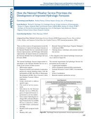
The U.S. Climate Change Science Program Chapter 1Abrupt climatechange is afundamentalcharacteristic of theclimate system.with the publication of climate records fromlong ice cores from the Greenland Ice Sheet(Fig. 1.1). Subsequent development of marineand terrestrial records (Fig. 1.1) that also resolvechanges on these short time scales has yieldeda wide variety of climate signals from highlyresolved and well-dated records from which thefollowing generalizations can be drawn:• abrupt climate change is a fundamentalcharacteristic of the climate system;• some past changes were subcontinental toglobal in extent;• the largest of these changes occurred duringtimes of greater-than-present global icevolume;• all components of the Earth’s climate system(ocean, atmosphere, cyrosphere, biosphere)were involved in the largest changes, indicatinga closely coupled system response withimportant feedbacks; and• many past changes can be linked to forcingsassociated with changes in sea-surfacetemperatures or increased freshwater fluxesfrom former ice sheets.These developments have led to an intensiveeffort by climate scientists to understand thepossible mechanisms of abrupt climate change.This effort is motivated by the fact that if suchlarge changes were to recur, they would havea potentially devastating impact on humansociety and natural ecosystems because of theinability of either to adapt on such short timescales. While past abrupt changes occurred inresponse to natural forcings, or were unforced,the prospect that human influences on the climatesystem may trigger similar abrupt changesin the near future (Broecker, 1997) adds furtherurgency to the topic.Significant progress has been made since thereport on abrupt climate change by the NationalResearch Council (NRC) in 2002 (NRC, 2002),and this report provides considerably greaterdetail and insight on many of these issues thanwas provided in the 2007 IntergovernmentalPanel on Climate Change (IPCC) FourthAssessment Report (AR4) (IPCC, 2007).New paleoclimate reconstructions have beendeveloped that provide greater understanding ofpatterns and mechanisms of past abrupt climatechange in the ocean and on land, and newobservations are further revealing unanticipatedrapid dynamical changes of modern glaciers, icesheets, and ice shelves as well as processes thatare contributing to these changes. Finally, improvementsin modeling of the climate systemhave further reduced uncertainties in assessingthe likelihood of an abrupt change. The presentreport reviews this progress.2. Definition of AbruptClimate ChangeWhat is meant by abrupt climate change? Severaldefinitions exist, with subtle but importantdifferences. Clark et al. (2002) defined abruptclimate change as “a persistent transition ofclimate (over subcontinental scale) that occurson the timescale of decades.” The NRC report“Abrupt Climate Change” (NRC, 2002) offeredtwo definitions of abrupt climate change. Amechanistic definition defines abrupt climatechange as occurring when “the climate systemis forced to cross some threshold, triggering atransition to a new state at a rate determinedby the climate system itself and faster thanthe cause.” This definition implies that abruptclimate changes involve a threshold or nonlinearfeedback within the climate system from onesteady state to another, but is not restrictiveto the short time scale (1–100 years) that hasclear societal and ecological implications.Accordingly, the NRC report also providedan impacts-based definition of abrupt climatechange as “one that takes place so rapidly andunexpectedly that human or natural systemshave difficulty adapting to it.” Finally, Overpeckand Cole (2006) defined abrupt climatechange as “a transition in the climate systemwhose duration is fast relative to the durationof the preceding or subsequent state.” Similarto the NRC’s mechanistic definition, thisdefinition transcends many possible time scales,and thus includes many different behaviors ofthe climate system that would have little orno detrimental impact on human (economic,social) systems and ecosystems.For this report, we have modified and combinedthese definitions into one that emphasizesboth the short time scale and the impact onecosystems. In what follows we define abruptclimate change as:10

Abrupt Climate Change-35Arctic temperatureFigure 1.1. Records of climate changefrom the time period 35,000 to 65,000years ago, illustrating how many aspectsof the Earth’s climate system have changedabruptly in the past. In all panels, theupward-directed gray arrows indicate thedirection of increase in the climate variablerecorded in these geologic archives(i.e., increase in temperature, increase inmonsoon strength, etc.). The upper panelshows changes in the oxygen-isotopiccomposition of ice (δ 18 O) from the GISP2Greenland ice core (Grootes et al., 1993).Isotopic variations record changes in temperatureof the high northern latitudes,with intervals of cold climate (more negativevalues) abruptly switching to intervalsof warm climate (more positive values),representing temperature increases of8 °C to 15 °C typically occurring withindecades (Huber et al., 2006). The nextpanel down shows a record of strength ofthe Indian monsoon, with increasing valuesof total organic carbon (TOC) indicatingan increase in monsoon strength (Schulzet al., 1998). This record indicates thatchanges in monsoon strength occurredat the same time as, and at similar ratesas, changes in high northern-latitude temperatures.The next panel down shows arecord of the biological productivity of thesurface waters in the southwest PacificOcean east of New Zealand, as recordedby the concentration of alkenones inmarine sediments (Sachs and Anderson,2005). This record indicates that large increasesin biological productivity of thesesurface waters occurred at the same timeas cold temperatures in high-northernδ 18 O (per mil)Alk (ng g -1 )δ 18 O (per mil)-55800200-36-41Indian monsoonOcean productivityWetland methaneproductionAntarctic temperature65 60 55 50 45 40 35Age (x 10 3 yr)latitudes and weakened Indian monsoon strength. The next panel down is a record of changes in theconcentration of atmospheric methane (CH 4 ) from the GISP2 ice core (Brook et al., 1996). As discussedin Chapter 5 of this report, methane is a powerful greenhouse gas, but the variations recorded were notlarge enough to have a significant effect on radiative forcing. However, these variations are important inthat they are thought to reflect changes in the tropical water balance that controls the distribution ofmethane-producing wetlands. Times of high-atmospheric methane concentrations would thus correspondto a greater distribution of wetlands, which generally correspond to warm high northern latitudes anda stronger Indian monsoon. The bottom panel is an oxygen-isotopic (δ 18 O) record of air temperaturechanges over the Antarctic continent (Blunier and Brook, 2001). In this case, warm temperatures overAntarctica correspond to cold high northern latitudes, weakened Indian monsoon and drier tropics, andgreat biological productivity of the southwestern Pacific Ocean.6TOC (%)0700CH 4(ppb)40011

The U.S. Climate Change Science Program Chapter 1A large-scale change in the climatesystem that takes place over a fewdecades or less, persists (or is anticipatedto persist) for at least a fewdecades, and causes substantialdisruptions in human and naturalsystems.3. ORGANIZATION OF REPORTSynthesis and Assessment Product 3.4 considersfour types of change documented in thepaleoclimate record that stand out as beingso rapid and large in their impact that theypose clear risks to the ability of society andecosystems to adapt. These changes are (i) rapiddecrease in ice sheet mass with resulting globalsea level rise; (ii) widespread and sustainedchanges to the hydrologic cycle that inducesdrought; (iii) changes in the Atlantic MeridionalOverturning Circulation (AMOC); and(iv) rapid release to the atmosphere of the potentgreenhouse gas methane, which is trapped inpermafrost and on continental slopes. Based onthe published scientific literature, each chapterexamines one of these types of change (sealevel, drought, AMOC, and methane), providinga detailed assessment of the likelihood of futureabrupt change as derived from reconstructionsof past changes, observations and modeling ofthe present physical systems that are subjectto abrupt change, and where possible, climatemodel simulations of future behavior of changesin response to increased GHG concentrations.In providing this assessment, we adopt theIPCC AR4 standard terms used to define thelikelihood of an outcome or result where thiscan be determined probabilistically (Box 1.1).4. ABRUPT CHANGE INSEA LEVELPopulation densities in coastal regions and onislands are about three times higher than theglobal average, with approximately 23% of theworld’s population living within 100 kilometers(km) distance of the coast and 99% probability>95% probability>90% probability>66% probability>50% probability33 to 66% probability

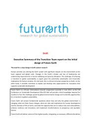
Abrupt Climate ChangeFigure 1.2. Portions (shown in red) of the Southeastern United States, Central America, and theCaribbean surrounding the Gulf of Mexico that would be inundated by a 6-meter sea level rise (fromRowley et al., 2007). Note that additional changes in the position of the coastline may occur in responseto erosion from the rising sea level.celerated to 3.1 ± 0.7 mm yr –1 , reflecting eithervariability on decadal time scales or an increasein the longer term trend. Relative to the period1961–2003, estimates of the contributions fromthermal expansion and from glaciers and icesheets indicate that increases in both of thesesources contributed to the acceleration in globalsea level rise that characterized the 1992–2003period (Bindoff et al., 2007).By the end of the 21st century, and in the absenceof ice-dynamical contributions, the IPCCAR4 projects sea level to rise by 0.28 ± 0.10 mto 0.42 ± 0.16 m in response to additional globalwarming, with the contribution from thermalexpansion accounting for 70–75% of this rise(Meehl et al., 2007). Projections for contributionsfrom ice sheets are based on models thatemphasize accumulation and surface meltingin controlling the amount of mass gained andlost by ice sheets (mass balance), with differentrelative contributions for the Greenland andAntarctic ice sheets. Because the increase inmass loss (ablation) is greater than the increasein mass gain (accumulation), the GreenlandIce Sheet is projected to contribute to a positivesea level rise and may melt entirely fromfuture global warming (Ridley et al., 2005). Incontrast, the Antarctic Ice Sheet is projected togrow through increased accumulation relativeto ablation and thus contribute to a negative sealevel rise. The net projected effect on globalsea level from these two differing ice-sheetresponses to global warming over the remainderof this century is to nearly cancel each other out.Accordingly, the primary contribution to sealevel rise from projected mass changes in theIPCC AR4 is associated with retreat of glaciersand ice caps (Meehl et al., 2007).Rahmstorf (2007) used the relation between20th century sea level rise and global meansurface temperature increase to predict a sealevel rise of 0.5 to 1.4 m above the 1990 level bythe end of the 21st century, considerably higherthan the projections by the IPCC AR4 (Meehlet al., 2007). Insofar as the contribution to 20thcentury sea level rise from melting land ice isthought to have been dominated by glaciers andice caps (Bindoff et al., 2007), the Rahmstorf(2007) projection does not include the possiblecontribution to sea level rise from ice sheets.Recent observations of startling changes atthe margins of the Greenland and Antarcticice sheets indicate that dynamic responsesRecent observationsof startling changesat the margins ofthe Greenlandand Antarctic icesheets indicate thatdynamic responsesto warming may playa much greater rolein the future massbalance of ice sheetsthan considered incurrent numericalprojections of sealevel rise.13

The U.S. Climate Change Science Program Chapter 1The primary factorthat raises concernsabout the potentialof future abruptchanges in sea levelis that large areasof modern icesheets are currentlygrounded below sealevel.to warming may play a much greater role inthe future mass balance of ice sheets thanconsidered in current numerical projectionsof sea level rise. Ice-sheet models used as thebasis for the IPCC AR4 numerical projectionsdid not include the physical processes thatmay be governing these dynamical responses,but if they prove to be significant to thelong-term mass balance of the ice sheets, sealevel projections will likely need to be revisedupwards substantially. By implicitly excludingthe potential contribution from ice sheets, theRahmstorf (2007) estimate will also likely needto be revised upwards if dynamical processescause future ice-sheet mass balance to becomemore negative.Chapter 2 of this report summarizes the availableevidence for recent changes in the mass ofglaciers and ice sheets. The Greenland Ice Sheetis losing mass and very likely on an acceleratedpath since the mid-1990s. Observations showthat Greenland is thickening at high elevations,because of an increase in snowfall, but thatthis gain is more than offset by an acceleratingmass loss at the coastal margins, with alarge component from rapidly thinning andaccelerating outlet glaciers. The mass balanceof the Greenland Ice Sheet during the periodwith good observations indicates that the lossincreased from 100 gigatons per year (Gt a –1 )(where 360 Gt of ice = 1 mm of sea level) in thelate 1990s to more than 200 Gt a –1 for the mostrecent observations in 2006.Determination of the mass budget of the Antarcticice sheet is not as advanced as that forGreenland. The mass balance for Antarcticaas a whole has experienced a net loss of about80 Gt a –1 in the mid-1990s, increasing to almost130 Gt a –1 in the mid-2000s. There is little surfacemelting in Antarctica, but substantial icelosses are occurring from West Antarctica andthe Antarctic Peninsula primarily in responseto changing ice dynamics.The record of past changes provides importantinsight to the behavior of large ice sheets duringwarming. At the last glacial maximum about21,000 years ago, ice volume and area wereabout 2.5 times modern. Deglaciation wasforced by warming from changes in the Earth’sorbital parameters, increasing greenhousegas concentrations, and attendant feedbacks.Deglacial sea level rise averaged 10 mm a –1 ,but with variations including two extraordinaryepisodes at 19,000 years ago (ka) and 14.5 kawhen peak rates potentially exceeded 50 mma –1 (Fairbanks, 1989; Yokoyama et al., 2000).Each of these “meltwater pulses” added theequivalent of 1.5 to 3 Greenland ice sheets(~10–20 m) to the oceans over a one- to fivecenturyperiod, clearly demonstrating thepotential for ice sheets to cause rapid and largesea level changes.The primary factor that raises concerns aboutthe potential of future abrupt changes in sealevel is that large areas of modern ice sheetsare currently grounded below sea level. Whereit exists, it is this condition that lends itself tomany of the processes that can lead to rapidice-sheet changes, especially with regard toatmosphere-ocean-ice interactions that mayaffect ice shelves and calving fronts of glaciersterminating in water (tidewater glaciers). Animportant aspect of these marine-based icesheets is that the beds of ice sheets groundedbelow sea level tend to deepen inland. Thegrounding line is the critical juncture thatseparates ice that is thick enough to remaingrounded from either an ice shelf or a calvingfront. In the absence of stabilizing factors, thisconfiguration indicates that marine ice sheetsare inherently unstable, whereby small changesin climate could trigger irreversible retreat ofthe grounding line.The amount of retreat clearly depends on howfar inland glaciers remain below sea level.Of greatest concern is the West Antarctic IceSheet, with 5 to 6 m sea level equivalent, wheremuch of the base of the ice sheet is grounded14

Abrupt Climate Changewell below sea level, with deeper trencheslying well inland of their grounding lines. Asimilar situation applies to the entire WilkesLand sector of East Antarctica. In Greenland,a number of outlet glaciers remain below sealevel, indicating that glacier retreat by thisprocess will continue for some time. A notableexample is Greenland’s largest outlet glacier,Jakobshavn Isbræ, which appears to tap intothe central region of Greenland that is belowsea level. Accelerated ice discharge is possiblethrough such outlet glaciers, but we consider thepotential for destabilization of the GreenlandIce Sheet by this mechanism to be very unlikely.The key requirement for stabilizing groundinglines of marine-based ice sheets appears to bethe presence of an extension of floating icebeyond the grounding line, referred to as an iceshelf. A thinning ice shelf results in ice-sheetungrounding, which is the main cause of the iceacceleration because it has a large effect on theforce balance near the ice front. Recent rapidchanges in marginal regions of both ice sheetsare characterized mainly by acceleration andthinning, with some glacier velocities increasingmore than twofold. Many of these glacieraccelerations closely followed reduction or lossof ice shelves. If glacier acceleration caused bythinning ice shelves can be sustained over manycenturies, sea level will rise more rapidly thancurrently estimated.Such behavior was predicted almost 30 yearsago by Mercer (1978) but was discounted asrecently as the IPCC Third Assessment Report(Church et al., 2001) by most of the glaciologicalcommunity based largely on results from prevailingmodel simulations. Considerable effortis now underway to improve the models, but itis far from complete, leaving us unable to makereliable predictions of ice-sheet responses to awarming climate if such glacier accelerationswere to increase in size and frequency.waters entering the cavities beneath ice shelves.Future changes in ocean circulation and oceantemperatures will produce changes in basalmelting, but the magnitude of these changes iscurrently neither modeled nor predicted.Another mechanism that can potentiallyincrease the sensitivity of ice sheets to climatechange involves enhanced flow of the ice overits bed due to the presence of pressurizedwater, a process known as sliding. Where suchbasal flow is enabled, total ice flow rates mayincrease by 1 to 10 orders of magnitude, significantlydecreasing the response time of an icesheet to a climate or ice-marginal perturbation.Recent data from Greenland show a high correlationbetween periods of heavy surface meltingand an increase in glacier velocity (Zwally et al.,2002). A possible cause for this relation is rapiddrainage of surface meltwater to the glacierbed, where it enhances lubrication and basalsliding. There has been a significant increasein meltwater runoff from the Greenland IceSheet for the 1998–2007 period compared tothe previous three decades (Fig. 1.3). Total meltarea is continuing to increase during the meltseason and has already reached up to 50% ofthe Greenland Ice Sheet; further increase inArctic temperatures will very likely continuethis process and will add additional runoff.Because water represents such an importantcontrol on glacier flow, an increase in meltwaterproduction in a warmer climate will likely havemajor consequences on flow rate and mass loss.A nonlinear response of ice-shelf melting toincreasing ocean temperatures is a central tenetin the scenario for abrupt sea-level rise arisingfrom ocean–ice-shelf interactions. Significantchanges in ice-shelf thickness are most readilycaused by changes in basal melting. The susceptibilityof ice shelves to high melt rates and tocollapse is a function of the presence of warm15

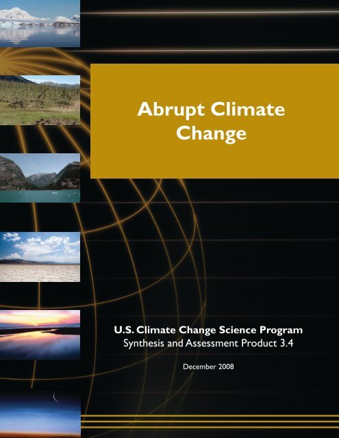
The U.S. Climate Change Science Program Chapter 11996 19983.00E+07Total Melt AreaApril - October20072007elted (km 2 )Area M2.50E+072.00E+07071987199119951998200220051.50E+071.00E+071983199219965.00E+061978 1983 1988 1993 1998 2003 2008YearKonrad Steffen and Russell Huff, CIRES, University of Colorado at BoulderFigure 1.3. The graph shows the total melt area 1979 to 2007 for the Greenland ice sheet derivedfrom passive microwave satellite data. Error bars represent the 95% confidence interval. The mapinserts display the area of melt for 1996, 1998, and the record year 2007 (from K. Steffen, CIRES,University of Colorado).Because sites of global deep water formationoccur immediately adjacent to the Greenlandand Antarctic ice sheets, any significant increasein freshwater fluxes from these ice sheetsmay induce changes in ocean heat transportand thus climate. This topic is addressed inChapter 4 of this report.SummaryThe Greenland and Antarctic Ice Sheets arelosing mass, likely at an accelerating rate. Muchof the loss from Greenland is by increasedsummer melting as temperatures rise, but anincreasing proportion of the combined massloss is caused by increasing ice discharge fromthe ice-sheet margins, indicating that dynamicalresponses to warming may play a much greaterrole in the future mass balance of ice sheetsthan previously considered. The interactionof warm waters with the periphery of the icesheets is very likely one of the most significantmechanisms to trigger an abrupt rise in globalsea level. The potentially sensitive regions forrapid changes in ice volume are thus likely thoseice masses grounded below sea level such asthe West Antarctic Ice Sheet or large glaciersin Greenland like the Jakobshavn Isbræ withan over-deepened channel (channel below sealevel, see Chapter 2, Fig. 2.10) reaching far inland.Ice-sheet models currently do not includethe physical processes that may be governingthese dynamical responses, so quantitativeassessment of their possible contribution to sealevel rise is not yet possible. If these processesprove to be significant to the long-term massbalance of the ice sheets, however, current sealevel projections based on present-generationnumerical models will likely need to be revisedsubstantially upwards.5. Abrupt Change in LandHydrologyMuch of the research on the climate responseto increased GHG concentrations, and mostof the public’s understanding of that work,has been concerned with global warming.Accompanying this projected globally uniformincrease in temperature, however, are spatially16

Abrupt Climate Changeheterogeneous changes in water exchange betweenthe atmosphere and the Earth’s surfacethat are expected to vary much like the currentdaily mean values of precipitation and evaporation(IPCC, 2007). Although projected spatialpatterns of hydroclimate change are complex,these projections suggest that many alreadywet areas are likely to get wetter and alreadydry areas are likely to get drier, while someintermediate regions on the poleward flanks ofthe current subtropical dry zones are likely tobecome increasingly arid.These anticipated changes will increase problemsat both extremes of the water cycle,stressing water supplies in many arid andsemi-arid regions while worsening flood hazardsand erosion in many wet areas. Moreover,the instrumental, historical, and prehistoricalrecord of hydrological variations indicates thattransitions between extremes can occur rapidlyrelative to the time span under consideration.Over the course of several decades, for example,transitions between wet conditions and dryconditions may occur within a year and canpersist for several years.Abrupt changes or shifts in climate that lead todrought have had major impacts on societiesin the past. Paleoclimatic data document rapidshifts to dry conditions that coincided withdownfall of advanced and complex societies.The history of the rise and fall of several empiresand societies in the Middle East between7000 and 2000 B.C. have been linked to abruptshifts to persistent drought conditions (Weissand Bradley, 2001). Severe drought leading tocrop failure and famine in the mid-8th centuryhas been suggested as cause for the declineand collapse of the Tang Dynasty (Yancheva etal., 2007) and the Classic Maya (Hodell et al.,1995). A more recent example of the impact ofsevere and persistent drought on society is the1930s Dust Bowl in the Central United States(Fig. 1.4), which led to a large-scale migrationof farmers from the Great Plains to the WesternUnited States. Societies in many parts of theworld today may now be more insulated to theimpacts of abrupt climate shifts in the form ofdrought through managed water resources andreservoir systems. Nevertheless, populationgrowth and over-allocation of scarce water suppliesin a number of regions have made societieseven more vulnerable to the impacts of abruptclimate change involving drought.Variations in water supply, in general, andprotracted droughts, in particular, are amongthe greatest natural hazards facing the UnitedStates and the globe today and in the foreseeablefuture. According to the National Climatic DataCenter, National Oceanic and Atmospheric Administration(NCDC, NOAA), over the periodfrom 1980 to 2006 droughts and heat waveswere the second most expensive natural disasterin the United States behind tropical storms.The annual cost of drought to the United Statesis estimated to be in the billions of dollars.Although there is much uncertainty in thesefigures, it is clear that drought leads to (1) croplosses, which result in a loss of farm incomeand an increase in Federal disaster relief fundsand food prices, (2) disruption of recreation andtourism, (3) increased fire risk and loss of lifeand property, (4) reduced hydroelectric energygeneration, and (5) enforced water conservationto preserve essential municipal water suppliesand aquatic ecosystems (Changnon et al., 2000;Pielke and Landsea, 1998; Ross and Lott, 2003).5.1. History of North AmericanDroughtIn Chapter 3 of this report, we examine NorthAmerican drought and its causes from theperspective of the historical record and, basedon paleoclimate records, the last 1,000 yearsand the last 10,000 years. This longer temporalperspective relative to the historical record allowsus to evaluate the natural range of droughtVariations in watersupply, in general,and protracteddroughts, inparticular, are amongthe greatest naturalhazards facing theUnited States andthe globe today andin the foreseeablefuture.Figure 1.4. Photograph showing a dust storm approaching Stratford,Texas, during the 1930s Dust Bowl. (NOAA Photo Library,Historic NWS collection).17

The U.S. Climate Change Science Program Chapter 1variability under a diverse range of meanclimatic conditions, including those similar tothe present.Instrumental precipitation and temperaturedata and tree-ring analyses provide sufficientinformation to identify six serious multiyeardroughts in western North America since 1856.Of these, the most famous is the “Dust Bowl”drought that included most of the 1930s decade(Fig. 1.4). The other two in the 20th century arethe severe drought in the Southwest from thelate 1940s to the late 1950s and the drought thatbegan in 1998 and is ongoing. Three droughts inthe middle to late 19th century occurred (withapproximate dates) from 1856 to 1865, from1870 to 1876, and from 1890 to 1896.Is the 1930s Dust Bowl drought the worst thatcan conceivably occur over North America?The instrumental and historical data only goback about 130 years with an acceptable degreeof spatial completeness over the United States,which does not provide us with enough timeto characterize the full range of hydroclimaticvariability that has happened in the past andcould conceivably happen in the future independentof any added effects due to greenhousewarming. To do so, we must look beyond thehistorical data to longer natural archives of pastclimate information to gain a better understandingof the past occurrence of drought and itsnatural range of variability.Much of what we have learned about the historyof North American drought over the past 1,000years is based on annual ring-width patternsof long-lived trees that are used to reconstructsummer drought based on the Palmer DroughtSeverity Index (PDSI). This information andother paleoclimate data have identified a periodof elevated aridity during the “Medieval ClimateAnomaly” (MCA) period (A.D. 900–1300)that included four particularly severe multidecadalmegadroughts (Fig. 1.5) (Cook et al.,2004). The range of annual drought variabilityduring this period was not any larger than thatseen after 1470, suggesting that the climateconditions responsible for these early droughtseach year were apparently no more extreme thanthose conditions responsible for droughts duringmore recent times. This can be appreciatedby noting that only 1 year of drought during theMCA was marginally more severe than the 1934Dust Bowl year. This suggests that the 1934event may be used as a worst-case scenario forhow severe a given year of drought can get overthe West. What sets these MCA megadroughtsFigure 1.5. Percent area affected by drought (PDSI

Abrupt Climate Changeapart from droughts of more modern times,however, is their duration, with droughts duringthe MCA lasting much longer than historicdroughts in the Western United States.The emphasis up to now has been on the semiaridto arid Western United States because thatis where the late-20th century drought beganand has largely persisted up to the presenttime. Yet, previous studies indicate that megadroughtshave also occurred in the importantcrop-producing states in the Midwest and GreatPlains as well (Stahle et al., 2007). In particular,a tree-ring PDSI reconstruction for the GreatPlains shows the MCA period with even morepersistent drought than the Southwest, but nowon a centennial time scale.Examination of drought history over the last11,500 years (referred to as the Holocene Epoch)is motivated by noting that the projected changesin both the radiative forcing and the resultingclimate of the 21st century far exceed thoseregistered by either the instrumental records ofthe past century or by geologic archives that canbe calibrated to derive climate (proxy records)of the past few millennia. In other words, all ofthe variations in climate over the instrumentalperiod and over the past millennia reviewedabove have occurred in a climate system whosecontrols have not differed much from those ofthe 20th century. Consequently, a longer termperspective is required to describe the behaviorof the climate system under controls as differentfrom those at present as those of the 21st centurywill be, and to assess the potential for abruptclimate changes to occur in response to gradualchanges in large-scale forcing.It is important to emphasize that the controlsof climate during the 21st century and duringthe Holocene differ from one another, and fromthose of the 20th century, in important ways.The major difference in controls of climatebetween the early 20th, late 20th, and 21stcentury is in atmospheric composition (withan additional component of land-cover change).In contrast, the major difference between thecontrols in the 20th and 21st centuries andthose in the early to middle Holocene is in thelatitudinal and seasonal distribution of solarradiation. Accordingly, climatic variationsduring the Holocene should not be thoughtof either as analogs for future climates or asexamples of what might be observable underpresent-day climate forcing if records werelonger, but instead should be thought of as theresult of a natural experiment within the climatesystem that features large perturbations of thecontrols of climate.The paleoclimatic record from North Americaindicates that drier conditions than presentcommenced in the mid-continent between 10and 8 thousand years ago (ka) (Webb et al.,1993), and ended after 4 ka. The variety of paleoenvironmentalindicators reflect the spatialextent and timing of these moisture variations,and in general suggest that the dry conditionsincreased in their intensity during the intervalfrom 11 ka to 8 ka, and then gave way to increasedmoisture after 4 ka. During the middleof this interval (around 6 ka) dry conditionswere widespread. Lake-status indicators at 6 kaindicate lower-than-present levels (and hencedrier-than-present conditions) across most ofthe continent, and quantitative interpretation ofpollen data shows a similar pattern of overallaridity, but again with some regional and localvariability, such as moister-than-presentconditions in the Southwestern United States(Williams et al., 2004). Although the region ofdrier-than-present conditions extends into theNortheastern United States and eastern Canada,most of the evidence for mid-Holocene drynessis focused on the mid-continent, in particular19

The U.S. Climate Change Science Program Chapter 1Empirical studiesand climate modelexperiments showthat droughts overNorth Americaand globallyare significantlyinfluenced by thestate of tropicalsea surfacetemperatures.the Great Plains and Midwest, where the evidencefor aridity is particularly clear.5.2. Causes of North AmericanDroughtEmpirical studies and climate model experimentsshow that droughts over North Americaand globally are significantly influenced by thestate of tropical sea surface temperatures (SSTs),with cool, persistent La Niña-like SSTs in theeastern equatorial Pacific frequently causingdevelopment of droughts over the SouthwesternUnited States and Northern Mexico. Climatemodels that have evaluated this linkage needonly prescribe small changes in SSTs, no morethan a fraction of a degree Celsius, to result inreductions in precipitation. It is the persistenceof the SST anomalies and associated moisturedeficits that creates serious drought conditions.In the Pacific, the SST anomalies presumablyarise naturally from dynamics similar to thoseassociated with the El Niño Southern Oscillation(ENSO) on time scales of a year to adecade (Newman et al., 2003). On long timescales, the dynamics that link tropical PacificSST anomalies to North American hydroclimateappear as analogs of higher frequencyphenomena associated with ENSO (Shin et al.,2006). In general, the atmospheric response toLa Niña-like conditions forces descent of airover western North America that suppressesprecipitation. In addition to the ocean influence,some modeling and observational estimatesindicate that soil-moisture feedbacks also influenceprecipitation variability.The causes of the MCA megadroughts appearto have similar origin to the causes of moderndroughts, which is consistent with the similarspatial patterns expressed by MCA and moderndroughts (Herweijer et al., 2007). In particular,modeling experiments indicate that thesemegadroughts may have occurred in response tocold tropical Pacific SSTs and warm subtropicalNorth Atlantic SSTs externally forced by highirradiance and weak volcanic activity (Mann etal., 2005; Emile-Geay et al., 2007). However,this result is tentative, and the exceptional durationof the droughts has not been adequatelyexplained, nor whether they also involvedforcing from SST changes in other ocean basins.Over longer time spans, the paleoclimaticrecord indicates that even larger hydrologicalchanges have taken place in response to pastchanges in the controls of climate that rival inmagnitude those predicted for the next severaldecades and centuries. These changes weredriven ultimately by variations in the Earth’sorbit that altered the seasonal and latitudinaldistribution of incoming solar radiation. Theclimate boundary conditions associated withthose changes were quite different from thoseof the past millennium and today, but they showthe additional range of natural variability andtruly abrupt hydroclimatic change that can beexpressed by the climate system.SummaryThe paleoclimatic record reveals dramaticchanges in North American hydroclimate overthe last millennium that were not associatedwith changes in greenhouse gases and humaninducedglobal warming. Accordingly, oneimportant implication of these results is thatbecause these megadroughts occurred underconditions not too unlike today’s, the UnitedStates still has the capacity to enter into aprolonged state of dryness even in the absenceof increased greenhouse-gas forcing.In response to increased concentration ofGHGs, the semi-arid regions of the Southwestare projected to dry in the 21st century, withthe model results suggesting, if they are correct,that the transition may already be underway(Seager et al., 2007). The drying in the Southwestis a matter of great concern because waterresources in this region are already stretched,new development of resources will be extremelydifficult, and the population (and thus demandfor water) continues to grow rapidly. Other subtropicalregions of the world are also expectedto dry in the near future, turning this featureof global hydroclimatic change into an internationalissue with potential impacts on migrationand social stability. The midcontinental U.S.Great Plains could also experience changes inwater supply impacting agricultural practices,grain exports, and biofuel production.20

Abrupt Climate Change6. Abrupt Change in theAtlantic MeridionalOverturning CirculationThe Atlantic Meridional Overturning Circulation(AMOC) is an important component ofthe Earth’s climate system, characterized bya northward flow of warm, salty water in theupper layers of the Atlantic, a transformation ofwater mass properties at higher northern latitudesof the Atlantic in the Nordic and LabradorSeas that induces sinking of surface waters toform deep water, and a southward flow of colderwater in the deep Atlantic (Fig. 1.6). Thereis also an interhemispherictransport of heat associatedwith this circulation, with heattransported from the SouthernHemisphere to the NorthernHemisphere. This ocean currentsystem thus transportsa substantial amount of heatfrom the Tropics and SouthernHemisphere toward the NorthAtlantic, where the heat isreleased to the atmosphere(Fig. 1.7).the instrumental record (based on the last ~130years) shows pronounced, multidecadal swingsin large-scale Atlantic temperature that may beat least partly a consequence of fluctuations inthe AMOC. Recent modeling and observationalanalyses have shown that these multidecadalshifts in Atlantic temperature exert a substantialinfluence on the climate system ranging frommodulating African and Indian monsoonal rainfallto tropical Atlantic atmospheric circulationconditions of relevance for hurricanes. AtlanticSSTs also influence summer climate conditionsover North America and Western Europe.Evidence from paleorecords suggests that therehave been large, decadal-scale changes in theAMOC, particularly during glacial times. Theseabrupt change events have had a profound impacton climate, both locally in the Atlantic andin remote locations around the globe (Fig. 1.1).Research suggests that these abrupt events wererelated to discharges of freshwater into theNorth Atlantic from surrounding land-based icesheets. Subpolar North Atlantic air temperaturechanges of more than 10 °C on time scales ofa decade or two have been attributed to theseabrupt change events.Changes in theAMOC have aprofound impacton many aspects ofthe global climatesystem.Changes in the AMOC havea profound impact on manyaspects of the global climatesystem. There is growing evidencethat fluctuations in Atlanticsea surface temperatures,hypothesized to be related tofluctuations in the AMOC,have played a prominent role insignificant climate fluctuationsaround the globe on a varietyof time scales. Evidence fromFigure 1.6. Schematic of the ocean circulation (from Kuhlbrodt et al., 2007) associated withthe global Meridional Overturning Circulation (MOC), with special focus on the Atlantic sectionof the flow (AMOC). The red curves in the Atlantic indicate the northward flow of water in theupper layers. The filled orange circles in the Nordic and Labrador Seas indicate regions wherenear-surface water cools and becomes denser, causing the water to sink to deeper layers of theAtlantic. The light blue curve denotes the southward flow of cold water at depth. See Chapter 4of this report for further explanation.21

The U.S. Climate Change Science Program Chapter 1Figure 1.7. Palm trees on Mullaghmore Head, County Sligo, Ireland, whichare symbolic of the relatively balmy climates of Ireland provided in part by theheat supplied from the Atlantic Meridional Overturning Circulation. Reprintedwith permission from http://www.a-wee-bit-of-ireland.com, copyright 2004.6.1. Uncertainties in Modelingthe AMOCAs with any projection of future behavior ofthe climate system, our understanding of theAMOC in the 21st century and beyond relies onnumerical models that simulate the importantphysical processes governing the overturningcirculation. An important test of model skill isto conduct transient simulations of the AMOCin response to the addition of freshwater andcompare with paleoclimatic data. Such a testrequires accurate, quantitative reconstructionsof the freshwater forcing, including its volume,duration, and location, plus the magnitudeand duration of the resulting reduction inthe AMOC. This information is not easy toobtain; coupled general circulation model(GCM) simulations of most events have beenforced with idealized freshwater pulses andcompared with qualitative reconstructions ofthe AMOC (e.g., Hewitt et al., 2006; Peltieret al., 2006; see also Stouffer et al., 2006).There is somewhat more information about thefreshwater pulse associated with an event 8,200years ago, but important uncertainties remain(Clarke et al., 2004; Meissner and Clark, 2006).Thus, simulations of such paleoclimatic eventsprovide important qualitative perspectives onthe ability of models to simulate the responseof the AMOC to forcing changes, but theirability to provide quantitative assessments islimited. Improvements in this area would bean important advance, but the difficulty inmeasuring even the current AMOC makes thistask daunting.Although numerical models show good skill inreproducing the main features of the AMOC,there are known errors that introduce uncertaintyin model results. Some of these model errors,particularly in temperature and heat transport,are related to the representation of westernboundary currents and deep-water overflowacross the Greenland-Iceland-Scotland ridge.Increasing the resolution of current coupledocean-atmosphere models to better addressthese errors will require an increase in computingpower by an order of magnitude. Suchhigher resolution offers the potential of morerealistic and robust treatment of key physicalprocesses, including the representation ofdeep-water overflows. Efforts are being madeto improve this model deficiency (Willebrand etal., 2001; Thorpe et al., 2004; Tang and Roberts,2005). Nevertheless, recent work by Spenceet al. (2008) using an Earth-system model of22

Abrupt Climate Changeintermediate complexity (EMIC) found thatthe duration and maximum amplitude of theircoupled model response to freshwater forcingshowed little sensitivity to increasing resolution.They concluded that the coarse-resolutionmodel response to boundary layer freshwaterforcing remained robust at finer horizontalresolutions.6.2. Future Changes in the AMOCA particular focus on the AMOC in Chapter 4 ofthis report is to address the widespread notion,both in the scientific and popular literature, thata major weakening or even complete shutdownof the AMOC may occur in response to globalwarming. This discussion is driven in part bymodel results indicating that global warmingtends to weaken the AMOC both by warmingthe upper ocean in the subpolar North Atlanticand through increasing the freshwater input(by more precipitation, more river runoff, andmelting inland ice) into the Arctic and NorthAtlantic. Both processes reduce the density ofthe upper ocean in the North Atlantic, therebystabilizing the water column and weakeningthe AMOC.It has been theorized that these processes couldcause a weakening or shutdown of the AMOCthat could significantly reduce the polewardtransport of heat in the Atlantic, thereby possiblyleading to regional cooling in the Atlanticand surrounding continental regions, particularlyWestern Europe. This mechanism can beinferred from paleodata and is reproduced atleast qualitatively in the vast majority of climatemodels (Stouffer et al., 2006). One of the mostmisunderstood issues concerning the futureof the AMOC under anthropogenic climatechange, however, is its often-cited potential tocause the onset of the next ice age. As discussedby Berger and Loutre (2002) and Weaver andHillaire-Marcel (2004), it is not possible forglobal warming to cause an ice age by thismechanism.In the past, there was disagreement in determiningwhich of the two processes governingupper-ocean density will dominate underincreasing GHG concentrations, but a recent11-model intercomparison project found that anMOC reduction in response to increasing GHGconcentrations was caused more by changes insurface heat flux than by changes in surfacefreshwater flux (Gregory et al., 2005). Nevertheless,different climate models show differentsensitivities toward an imposed freshwaterflux (Gregory et al., 2005). It is therefore notfully clear to what degree salinity changes willaffect the total overturning rate of the AMOC.In addition, by today’s knowledge, it is hardto assess how large future freshwater fluxesinto the North Atlantic might be. This is dueto uncertainties in modeling the hydrologicalcycle in the atmosphere, in modeling the sea-icedynamics in the Arctic, as well as in estimatingthe melting rate of the Greenland ice sheet (seeChapter 2 of this report).It is important to distinguish between anAMOC weakening and an AMOC collapse.Historically, coupled models that eventuallylead to a collapse of the AMOC under globalwarming scenarios have fallen into two categories:(1) coupled atmosphere-ocean generalcirculation models (AOGCMs) that requiredad hoc adjustments in heat or moisture fluxesto prevent them from drifting away from observations,and (2) intermediate-complexitymodels with longitudinally averaged oceancomponents. Current AOGCMs used in theIPCC AR4 assessment typically do not use fluxadjustments and incorporate improved physicsand resolution. When forced with plausibleestimates of future changes in greenhousegases and aerosols, these newer models projecta gradual 25–30% weakening of the AMOC,but not an abrupt change or collapse. Althougha transient collapse with climatic impacts onthe global scale can always be triggered inmodels by a large enough freshwater input (e.g.,Vellinga and Wood, 2007), the magnitude ofthe required freshwater forcing is not currentlyviewed as a plausible estimate of the future. Inaddition, many experiments have been conductedwith idealized forcing changes, in whichatmospheric CO 2 concentration is increased at arate of 1%/year to either two times or four timesthe preindustrial levels and held fixed thereafter.In virtually every simulation, the AMOCreduces but recovers to its initial strength whenthe radiative forcing is stabilized at two timesor four times the preindustrial levels.Perhaps more important for 21st century climatechange is the possibility for a rapid transitionOne of the mostmisunderstoodissues concerningthe future of theAMOC underanthropogenicclimate change is itsoften-cited potentialto cause the onsetof the next ice age.23

The U.S. Climate Change Science Program Chapter 1After carbon dioxide(CO 2 ), methane(CH 4 ) is the nextmost importantgreenhouse gas thathumans directlyinfluence.to seasonally ice-free Arctic conditions. Inone climate model simulation, a transitionfrom conditions similar to pre-2007 levels toa near-ice-free September extent occurred in adecade (Holland et al., 2006). Increasing oceanheat transport was implicated in this simulatedrapid ice loss, which ultimately resulted fromthe interaction of large, intrinsic variability andanthropogenically forced change. It is notablethat climate models are generally conservativein the modeled rate of Arctic ice loss ascompared to observations (Stroeve et al., 2007;Figure 1-3), suggesting that future ice retreatcould occur even more abruptly than simulated.This nonlinear response occurs because seaice has a strong inherent threshold in that itsexistence depends on the freezing temperatureof seawater. Additionally, strong positive feedbacksassociated with sea ice act to accelerate itschange. The most notable of these is the positivesurface albedo feedback in which changes in icecover and surface properties modify the surfacereflection of solar radiation. For example, in awarming climate, reductions in ice cover exposethe dark underlying ocean, allowing more solarradiation to be absorbed. This enhances thewarming and leads to further ice melt. Becausethe AMOC interacts with the circulation of theArctic Ocean at its northern boundary, futurechanges in the AMOC and its attendant heattransport thus have the potential to furtherinfluence the future of sea ice.SummaryOur analysis indicates that it is very likely thatthe strength of the AMOC will decrease overthe course of the 21st century. In models wherethe AMOC weakens, warming still occursdownstream over Europe due to the radiativeforcing associated with increasing greenhousegases. No model under plausible estimates offuture forcing exhibits an abrupt collapse of theMOC during the 21st century, even accountingfor estimates of accelerated Greenland ice sheetmelting. We conclude that it is very unlikely thatthe AMOC will abruptly weaken or collapseduring the course of the 21st century. Basedon available model simulations and sensitivityanalyses, estimates of maximum Greenland icesheet melting rates, and our understanding ofmechanisms of abrupt climate change from thepaleoclimatic record, we further conclude that itis unlikely that the AMOC will collapse beyondthe end of the 21st century as a consequence ofglobal warming, although the possibility cannotbe entirely excluded.The above conclusions depend upon our understandingof the climate system and on theability of current models to simulate the climatesystem. An abrupt collapse of the AMOC in the21st century would require either a sensitivityof the AMOC to forcing that is far greaterthan current models suggest or a forcing thatgreatly exceeds even the most aggressive ofcurrent projections (such as extremely rapidmelting of the Greenland ice sheet). While weview these as very unlikely, we cannot excludeeither possibility. Further, even if a collapse ofthe AMOC is very unlikely, the large climaticimpacts of such an event, coupled with thesignificant climate impacts that even decadalscale AMOC fluctuations induce, argue for astrong research effort to develop the observations,understanding, and models required topredict more confidently the future evolutionof the AMOC.7. Abrupt Change inAtmospheric MethaneConcentrationAfter carbon dioxide (CO 2 ), methane (CH 4 ) isthe next most important greenhouse gas thathumans directly influence. Methane is a potentgreenhouse gas because it strongly absorbsterrestrial infrared (IR) radiation. Methane’satmospheric abundance has more than doubledsince the start of the Industrial Revolution(Etheridge et al., 1998; MacFarling Meure etal., 2006), amounting to a total contribution toradiative forcing over this time of ~0.7 watts24

Abrupt Climate Changeper square meter (W m –2 ), or nearly half ofthat resulting from parallel increase in theatmospheric concentration of CO 2 (Hansen andSato, 2001). Additionally, CO 2 produced by CH 4oxidation is equivalent to ~6% of CO 2 emissionsfrom fossil fuel combustion. Over a 100-yeartime horizon, the direct and indirect effects onradiative forcing from emission of 1 kg CH 4 are25 times greater than for emission of 1 kg CO 2(IPCC, 2007). On shorter time scales, methane’simpact on radiative forcing is higher.The primary geological reservoirs of methanethat could be released abruptly to theatmosphere are found in ocean sediments andterrestrial soils as methane hydrate. Methanehydrate is a solid in which methane moleculesare trapped in a lattice of water molecules(Fig. 1.8). On Earth, methane hydrate formsunder high pressure–low temperature conditionsin the presence of sufficient methane.These conditions are most often found inrelatively shallow marine sediments on continentalmargins but also in some high-latitudesoils (Kvenvolden, 1993). Estimates of thetotal amount of methane hydrate vary widely,from 500 to 10,000 gigatons of carbon (GtC)total stored as methane in hydrates in marinesediments, and 7.5–400 GtC in permafrost(both figures are uncertain). The total amountof carbon in the modern atmosphere is ~810GtC, but the total methane content of theatmosphere is only ~4 GtC (Dlugokencky etal., 1998). Therefore, even a release of a smallportion of the methane hydrate reservoir to theatmosphere could have a substantial impact onradiative forcing.There is little evidence to support massivereleases of methane from marine or terrestrialhydrates in the past. Evidence from the ice corerecord indicates that abrupt shifts in methaneconcentration have occurred in the past 110,000years (Brook et al., 1996), but the concentrationchanges during these events were relativelysmall. Farther back in geologic time, an abruptwarming at the Paleocene-Eocene boundaryabout 55 million years ago has been attributedby some to a large release of methane to theatmosphere.Concern about future abrupt release in atmosphericmethane stems largely from thepossibility that the massive amounts of methanepresent as solid methane hydrate in ocean sedimentsand terrestrial soils may become unstablein the face of global warming. Warming orrelease of pressure can destabilize methanehydrate, forming free gas that may ultimatelybe released to the atmosphere (Fig. 1.9).The processes controlling hydrate stabilityand gas transport are complex, and only partlyunderstood. In Chapter 5 of this report, threecategories of mechanisms are consideredas potential causes of abrupt increases inatmospheric methane concentration in the nearfuture. These are summarized in the following.Figure 1.8. Clathrate hydrates are inclusion compoundsin which a hydrogen-bonded water framework—the hostlattice—traps “guest” molecules (typically gases) within icecages. The gas and water do not chemically bond, but interactthrough weak van der Waals forces, with each gas molecule—or cluster of molecules in some cases—confined to a singlecage. Clathrates typically crystallize into one of the threemain structures illustrated here. As an example, structure Iis composed of two types of cages: dodecahedra, 20 watermolecules arranged to form 12 pentagonal faces (designated5 12 ), and tetrakaidecahedra, 24 water molecules that form 12pentagonal faces and two hexagonal ones (5 12 6 2 ). Two 5 12 cagesand six 5 12 6 2 cages combine to form the unit cell. The picturedstructure I illustrates the water framework and trapped gasmolecules (from Mao et al.; used with permission, copyright2007, American Institute of Physics). See Chapter 5 of thisreport for further explanation.25

The U.S. Climate Change Science Program Chapter 1On the time scale of the coming century, it islikely that most of the marine hydrate reservoirwill be insulated from anthropogenic climatechange. The exception is in shallow oceansediments where methane gas is focused bysubsurface migration. These deposits will verylikely respond to anthropogenic climate changewith an increased background rate of sustainedmethane release, rather than an abrupt release.7.2. Destabilization of PermafrostHydratesHydrate deposits at depth in permafrost soilsare known to exist, and although their extentis uncertain, the total amount of methane inpermafrost hydrates appears to be much smallerthan in marine sediments. Surface warmingeventually would increase melting rates ofpermafrost hydrates. Inundation of some depositsby warmer seawater and lateral invasionof the coastline are also concerns and may bemechanisms for more rapid change.Figure 1.9. A piece of methane clathrate displays itspotential as an energy source. As the compound melts,released gas feeds the flame and the ice framework dripsoff as liquid water. Inlay shows the clathrate structure.Source: U.S. Geological Survey.7.1. Destabilization of MarineMethane HydratesThis issue is probably the most well knowndue to extensive research on the occurrence ofmethane hydrates in marine sediments, and thelarge quantities of methane apparently presentin this solid phase in primarily continentalmargin marine sediments. Destabilizationof this solid phase requires mechanisms forwarming the deposits and/or reducing pressureon the appropriate time scale, transport of freemethane gas to the sediment-water interface,and transport through the water column to theatmosphere (Archer, 2007). Warming of bottomwaters, slope failure, and their interaction arethe most commonly discussed mechanisms forabrupt release. However, bacteria are efficient atconsuming methane in oxygen-rich sedimentsand the ocean water column, and there are anumber of physical impediments to abruptrelease from marine sediments.Destabilization of hydrates in permafrostby global warming is unlikely over the nextfew centuries (Harvey and Huang, 1995). Nomechanisms have been proposed for the abruptrelease of significant quantities of methanefrom terrestrial hydrates (Archer, 2007). Slowand perhaps sustained release from permafrostregions may occur over decades to centuriesfrom mining extraction of methane from terrestrialhydrates in the Arctic (Boswell, 2007),over decades to centuries from continued erosionof coastal permafrost in Eurasia (Shakovaet al., 2005), and over centuries to millenniafrom the propagation of any warming 100 to1,000 meters down into permafrost hydrates(Harvey and Huang, 1995).7.3. Changes in Wetland Extentand Methane ProductivityAlthough a destabilization of either the marineor terrestrial methane hydrate reservoirs is themost likely pathway for an abrupt increasein atmospheric methane concentration, thepotential exists for a more gradual, but substantial,increase in natural methane emissionsin association with projected changes inclimate. The most likely region to experience adramatic change in natural methane emission26

Abrupt Climate Changeis the northern high latitudes, where there isincreasing evidence for accelerated warming,enhanced precipitation, and widespread permafrostthaw which could lead to an expansion ofwetland areas into organic-rich soils that, giventhe right environmental conditions, would befertile areas for methane production (Jorgensonet al., 2001, 2006).Tropical wetlands are a stronger methane sourcethan boreal and arctic wetlands and will likelycontinue to be over the next century, duringwhich fluxes from both regions are expected toincrease. However, several factors that differentiatenorthern wetlands from tropical wetlandsmake them more likely to experience a largerincrease in fluxes.The balance of evidence suggests that anticipatedchanges to northern wetlands in responseto large-scale permafrost degradation, thermokarstdevelopment, a positive trend in waterbalance in combination with substantial soilwarming, enhanced vegetation productivity,and an abundant source of organic matter willvery likely drive a sustained increase in CH 4emissions from the northern latitudes duringthe 21st century. A doubling of northern CH 4emissions could be realized fairly easily. Muchlarger increases cannot be discounted.SummaryThe prospect of a catastrophic release ofmethane to the atmosphere as a result ofanthropogenic climate change appears very unlikely.However, the carbon stored as methanehydrate and as potential methane in the organiccarbon pool of northern (and tropical) wetlandsoils is likely to play a role in future climatechange. Changes in climate, including warmertemperatures and more precipitation in someregions, particularly the Arctic, will very likelygradually increase emission of methane fromboth melting hydrates and natural wetlands. Themagnitude of this effect cannot be predictedwith great accuracy yet, but is likely to be atleast equivalent to the current magnitude ofmany anthropogenic sources.27

2CHAPTERAbrupt Climate ChangeRapid Changes in Glaciers andIce Sheets and their Impacts onSea LevelLead Author: konrad Steffen,* Cooperative Institute for Research inEnvironmental Sciences, University of ColoradoContributing Authors: Peter U. Clark,* Department ofGeosciences, Oregon State Universityj. Graham Cogley, Department of Geography, Trent University,CanadaDavid Holland, Courant Institute of Mathematical Sciences, New YorkUniversityShawn Marshall,* Department of Geography, University of Calgary,CanadaEric Rignot, School of Physical Sciences, University of California-Irvine, NASA Jet Propulsion Laboratory, and Centro de EstudiosCientifi cos, Valdivia, ChileRobert Thomas, EG&G Services, NASA Goddard Space Flight Center,Wallops Flight Facility, and Centro de Estudios Cientifi cos, Valdivia,Chile* SAP 3.4 Federal Advisory Committee memberkEy FINDINGS• Since the mid-19th century, small glaciers (sometimes called “glaciers and ice caps;” see Box 2.1 fordefinitions) have been losing mass at an average rate equivalent to 0.3 to 0.4 millimeters per year of sealevel rise.• The best estimate of the current (2007) mass balance of small glaciers is about –400 gigatons per year(Gt a –1 ), or nearly 1.1 millimeters sea level equivalent per year.• The mass balance loss of the Greenland Ice Sheet during the period with good observations increasedfrom 100 Gt a –1 in the mid-1990s to more than 200 Gt a –1 for the most recent observations in 2006.Much of the loss is by increased summer melting as temperatures rise, but an increasing proportion isby enhanced ice discharge down accelerating glaciers.• The mass balance for Antarctica is a net loss of about 80 Gt a –1 in the mid-1990s, increasing to almost130 Gt a –1 in the mid-2000s. There is little surface melting in Antarctica, and the substantial ice lossesfrom West Antarctica and the Antarctic Peninsula are very likely caused by increasing ice discharge asglacier velocities increase.• During the last interglacial period (~120 thousand years ago) with similar carbon dioxide levels to preindustrialvalues and arctic summer temperatures up to 4 °C warmer than today, sea level was 4–6 metersabove present. The temperature increase during the Eamian was the result of orbital changes of the sun.During the last two deglaciations, sea level rise averaged 10–20 millimeters per year with large “meltwaterfluxes” exceeding sea level rise of 50 millimeters per year lasting several centuries.• The potentially sensitive regions for rapid changes in ice volume are those with ice masses groundedbelow sea level such as the West Antarctic Ice Sheet, with 5 to 6 meters sea level equivalent, or largeglaciers in Greenland like the Jakobshavn Isbræ, also known as Jakobshavn Glacier and Sermeq Kujalleq(in Greenlandic), with an over-deepened channel (channel below sea level, see Figure 2.10) reaching farinland; total breakup of Jakobshavn Isbræ ice tongue in Greenland, as well as other tidewater glaciersand ice cap outlets, was preceded by its very rapid thinning.29

The U.S. Climate Change Science Program Chapter 2• Several ice shelves in Antarctica are thinning, and their area declined by more than 13,500 squarekilometers in the last 3 decades of the 20th century, punctuated by the collapse of the Larsen A andLarsen B ice shelves, soon followed by several-fold increases in velocities of their tributary glaciers.• The interaction of warm waters with the periphery of the large ice sheets represents a strongpotential cause of abrupt change in the big ice sheets, and future changes in ocean circulation andocean temperatures will very likely produce changes in ice-shelf basal melting, but the magnitude ofthese changes cannot currently be modeled or predicted. Moreover, calving, which can originate infractures far back from the ice front, and ice-shelf breakup, are very poorly understood.• Existing models suggest that climate warming would result in increased melting from coastal regionsin Greenland and an overall increase in snowfall. However, they are incapable of realistically simulatingthe outlet glaciers that discharge ice into the ocean and cannot predict the substantial acceleration ofsome outlet glaciers that we are already observing.CHAPTER 2. RECOMMENDATIONS• Reduce uncertainties in estimates of mass balance. This includes continuing mass-balancemeasurements on small glaciers and completing the World Glacier Inventory.• Maintain climate networks on ice sheets to detect regional climate change and calibrateclimate models.• Derive better measurements of glacier and ice-sheet topography and velocity throughimproved observation of glaciers and ice sheets. This includes utilizing existing satelliteinterferometric synthetic aperture radar (InSAR) data to measure ice velocity.• Use observations of the time-varying gravity field from satellites to estimate changes in icesheet mass.• Survey changes in ice-sheet topography using tools such as satellite radar (e.g., Envisat andCryosat-2), laser (e.g., ICESat-1/2), and wide-swath altimeters.• Monitor the polar regions with numerous satellites at various wavelengths to detectchange and to understand processes responsible for the accelerated ice loss of ice sheets,the disintegration of ice shelves, and the reduction of sea ice. It is the integrated satellitedata evaluation that provides the tools and understanding to model the future response ofcryospheric processes to climate change.• Utilize aircraft observations of surface elevation, ice thickness, and basal characteristics toensure that such information is acquired at high spatial resolution along specific routes, suchas glacier flow lines, and along transects close to the grounding lines.• Improve coverage of longer term (centennial to millennial) records of ice sheet and oceanhistory from geological observations.• Support field, theoretical, and computational investigations of physical processes beneath andalong ice shelves and beneath glaciers, especially near to the grounding lines of the latter, withthe goal of understanding recent increases in mass loss.• Develop ice-sheet models on par with current models of the atmosphere and ocean. Particulareffort is needed with respect to the modeling of ocean/ice-shelf interactions and physicalprocesses, of surface mass balance from climatic information, and of all (rather than just some,as now) of the forces which drive the motion of the ice.30

Abrupt Climate Change1. Summary1.1 PaleorecordThe most recent time with no appreciable iceon the globe was 35 million years ago duringa period when the atmospheric carbon dioxide(CO 2 ) was 1,250 ± 250 parts per million byvolume (ppmV) and a sea level 73 meters (m)higher than today. During the last interglacialperiod (~120 thousand years ago, ka) withsimilar CO 2 levels to pre-industrial valuesand arctic summer temperatures warmer thantoday, sea level was 4–6 m above present. Mostof that sea level rise (SLR) is believed to haveoriginated from the Greenland Ice Sheet, but therate of SLR is unknown. Sea level rise averaged10–20 millimeters per year (mm a –1 ) during thelast two deglaciation periods (130–116 ka and21–14 ka, respectively), with large “meltwaterfluxes” with rates of SLR exceeding 50 mm a –1lasting several centuries (Fairbanks, 1989;Rohling et al., 2008). Each of these meltwaterfluxes added 1.5–3 times the volume of thecurrent Greenland Ice Sheet (7 m) to the oceans.The cause, ice-sheet source, and mechanism ofthe meltwater fluxes are not well understood,yet the rapid loss of ice must have had an effecton ocean circulation resulting in a forcing ofthe global climate.1.2 Ice SheetsRapid changes in ice-sheet mass have surelycontributed to abrupt changes in climate andsea level in the past. The mass balance lossof the Greenland Ice Sheet increased in thelate 1990s to 100 gigatons per year (Gt a –1 ) oreven more than 200 Gt a –1 for the most recentobservations in 2006. It is extremely likely thatthe Greenland Ice Sheet islosing mass and very likelyon an accelerated path sincethe mid-1990s. The massbalance for Antarctica is anet loss of about 80 Gt a –1in the mid-1990s, increasingto almost 130 Gt a –1 inthe mid-2000s. The largestlosses are concentratedalong the Amundsen andBellinghausen sectors ofWest Antarctica and thenorthern tip of the AntarcticPeninsula. The potentiallysensitive regions for rapid changes in ice volumeare those with ice masses grounded below sealevel such as the West Antarctic Ice Sheet, with7 m sea level equivalent (SLE), or large glaciersin Greenland like the Jakobshavn, also knownas Jakobshavn Isbræ and Sermeq Kujalleq (inGreenlandic), with an over-deepened channelreaching far inland. There are large massbudgetuncertainties from errors in both snowaccumulation and calculated ice losses forAntarctica (~ ± 160 Gt a –1 ) and for Greenland(~ ± 35 Gt a –1 ). Mass-budget uncertainties fromaircraft or satellite observations (i.e., radar altimeter,laser altimeter, gravity measurements)are similar in magnitude. Most climate modelssuggest that climate warming would resultin increased melting from coastal regions inGreenland and an overall increase in snowfall.However, they do not predict the substantialacceleration of some outlet glaciers that we areobserving. This results from a fundamentalweakness in the existing models, which areincapable of realistically simulating the outletglaciers that discharge ice into the ocean.Observations show that Greenland is thickeningat high elevations, because of the increase insnowfall, which was predicted, but that thisgain is more than offset by an accelerating massloss, with a large component from rapidly thinningand accelerating outlet glaciers. Althoughthere is no evidence for increasing snowfallover Antarctica, observations show that somehigher elevation regions are also thickening,likely as a result of high interannual variabilityin snowfall. There is little surface melting inAntarctica, and the substantial ice losses fromWest Antarctica and the Antarctic Peninsula areThe potentiallysensitive regions forrapid changes in icevolume are thosewith ice massesgrounded below sealevel such as theWest Antarctic IceSheet, with 7 m sealevel equivalent.31

The U.S. Climate Change Science Program Chapter 2the main eventual constraint on mass balancewill be exhaustion of the supply of ice fromglaciers, which may take place in as little as50–100 years.Recent observationsof the ice sheetshave shownthat changes indynamics can occurfar more rapidlythan previouslysuspected.32very likely caused by increased ice dischargeas velocities of some glaciers increase. This isof particular concern in West Antarctica, wherebedrock beneath the ice sheet is deep belowsea level, and outlet glaciers are to some extent“contained” by the ice shelves into which theyflow. Some of these ice shelves are thinning,and some have totally broken up, and these arethe regions where the glaciers are acceleratingand thinning most rapidly.1.3 Small GlaciersWithin the uncertainty of the measurements,the following generalizations are justifiable.Since the mid-19th century, small glaciers havebeen losing mass at an average rate equivalentto 0.3–0.4 mm a –1 of sea level rise. The ratehas varied. There was a period of reducedloss between the 1940s and 1970s, with theaverage rate approaching zero in about 1970.We know with very high confidence that ithas been accelerating. The best estimate of thecurrent (2007) mass balance is near to –380to –400 Gt a –1 , or nearly 1.1 mm SLE a –1 ; thismay be an underestimate if, as suspected, theinadequately measured rate of loss by calvingoutweighs the inadequately measured rate ofgain by “internal” 2 accumulation. Our physicalunderstanding allows us to conclude that ifthe net gain of radiative energy at the Earth’ssurface continues to increase, then so willthe acceleration of mass transfer from smallglaciers to the ocean. Rates of loss observed sofar are small in comparison with rates inferredfor episodes of abrupt change during the lastfew hundred thousand years. In a warmer world2Refeezing at depth of percolating meltwater inspring and summer, and of retained capillary waterduring winter. Inability to measure these gains leadsto a potentially significant systematic error in the netmass balance.1.4 Causes of ChangePotential causes of the observed behavior ofice bodies include changes in snowfall and/or surface melting, long-term response to pastchanges in climate, and changes in ice dynamics.Smaller glaciers appear to be most sensitiveto radiatively induced changes in melting rate,but this may be because of inadequate attentionto the dynamics of tidewater glaciers (see Box2.1 for definitions). Recent observations of theice sheets have shown that changes in dynamicscan occur far more rapidly than previouslysuspected. There has been a significant increasein meltwater production on the Greenland IceSheet for the 1998–2003 time period comparedto the previous three decades, but this loss waspartly compensated by increased precipitation.Total melt area is continuing to increase duringsummer and fall and has already reached upto 50% of the Greenland Ice Sheet; furtherincrease in arctic temperatures will continuethis process and will add additional runoff.Recent rapid changes in marginal regions ofboth ice sheets show mainly acceleration andthinning, with some glacier velocities increasingmore than twofold. Most of these glacieraccelerations closely followed reduction or lossof ice shelves. Total breakup of JakobshavnIsbræ ice tongue in Greenland was preceded byits very rapid thinning. Thinning of more than1 meter per year (m a –1 ), and locally more than5 m a –1 , was observed during the past decadefor many small ice shelves in the Amundsen Seaand along the Antarctic Peninsula. Significantchanges in ice shelf thickness are most readilycaused by changes in basal melting. Recentdata show a high correlation between periodsof heavy surface melting and increase in glaciervelocity. A possible cause is rapid meltwaterdrainage to the glacier bed, where the waterenhances lubrication of basal sliding. Althoughno seasonal changes in the speeds were foundfor the rapid glaciers that discharge most icefrom Greenland, meltwater remains an essentialcontrol on glacier flow, and an increase inmeltwater production in a warmer climate couldlikely have major consequences of increasedflow rates and ice mass loss.

The U.S. Climate Change Science Program Chapter 2Application of this strategy to the retreat ofthe West Antarctic Ice Sheet (WAIS) from itsLGM position provides important context forunderstanding current ice dynamics. Conway etal. (1999) dated recession of the WAIS groundingline in the Ross Sea embayment and foundthat modern grounding-line retreat is part of anongoing recession that has been underway forthe last ~9,000 years. Stone et al. (2003) took aslightly different approach to evaluating WAISdeglaciation whereby they determined the rateof lowering of the ice-sheet surface by datingrecessional features preserved on a mountainslope that projected upward through the icesheet. Their results complemented those ofConway et al. (1999) in showing ice-sheet thinningfor the last ~10,000 years that may still beunderway. These results are important not onlyin providing constraints on long-term changesagainst which to evaluate short-term controls onice-sheet change but also in providing importantbenchmarks for modeling ice-sheet evolution.Nevertheless, the spatial coverage of these datafrom Antarctica remains limited, and additionalsuch constraints are needed.2. What is the Record ofPast Changes in Ice Sheetsand Global Sea Level?2.1 Reconstructing Past Changesin Ice SheetsThere are several methods available to reconstructpast changes in ice-sheet area and mass,each with its own strengths and shortcomings.Terrestrial records provide information offormer ice-sheet extent, whereby temporarystabilization of an ice margin may be recordedby an accumulation of sediment (moraine)that may be dated by isotopic methods (e.g.,10Be, 14 C, etc.). These records are important inidentifying the last maximum extent and retreathistory of an ice sheet (e.g., Dyke, 2004), butmost terrestrial records of glaciation prior to theLast Glacial Maximum (LGM) ~21,000 yearsago have been removed by erosion, limitingthe application of these records to times sincethe LGM. Moreover, in most cases they onlyprovide information on extent but not thickness,so that potential large changes in volume are notnecessarily captured by these records.Another strategy for constraining past ice-sheethistory is based on the fact that the weight of icesheets results in isostatic compensation of theunderlying solid Earth, generally referred to asglacial isostatic adjustment (GIA). Changes inice-sheet mass cause vertical motions that maybe recorded along a formerly glaciated coastlinewhere the global sea level serves as a datum.Since changes in ice mass will also causechanges in local (due to gravity) and global (dueto volume) sea level, the changes in sea levelat a particular coastline record the differencebetween vertical motions of the land and sea,commonly referred to as near-field relative sealevel (RSL) changes. Models that incorporatethe physical properties of the solid Earth invertthe RSL records to determine the ice-loadinghistory required to produce the isostatic adjustmentpreserved by these records (e.g., Peltier,2004). Because of the scarcity of such near-fieldRSL sites from the Antarctic continent, Ivinsand James (2005) constructed a history of Antarcticice-mass changes from geologic evidenceof ice-margin and ice-thickness changes, suchas described above (Conway et al., 1999; Stoneet al., 2003). This ice-load history was then usedto derive a model of present-day GIA.34

Abrupt Climate ChangeRegardless how it is derived, the GIA processmust be accounted for when using satellitealtimetry and gravity data to infer changes inice mass (e.g., Velicogna and Wahr, 2006b)(see Sec. 3). Given the poor constraints fromnear-field RSL records and geologic records(and their dating) of ice limits and thicknessesfor Antarctica, as well as uncertaintiesin properties of the solid Earth used in thesemodels, uncertainty in this GIA correction islarge (Velicogna and Wahr, 2006b; Barlettaet al., 2008). Accordingly, improvements inunderstanding present-day GIA are requiredto improve ice-mass estimates from altimetryand gravity data.2.2 Reconstructing Past Sea LevelSea level changes that occur locally, due toregional uplift or subsidence, relative to globalsea level are referred to as relative sea level(RSL) changes, whereas changes that occurglobally are referred to as eustatic changes.On time scales greater than 100,000 years,eustatic changes occur primarily from changesin ocean-basin volume induced by variationsin the rate of sea-floor spreading. On shortertime scales, eustatic changes occur primarilyfrom changes in ice volume, with secondarycontributions (order of 1 m) associated withchanges in ocean temperature or salinity(steric changes). Changes in global ice volumealso cause global changes in RSL in responseto the redistribution of mass between landto sea and attendant isostatic compensationand gravitational reequilibration. This GIAprocess must be accounted for in determiningeustatic changes from geomorphic records offormer sea level. Because the effects of the GIAprocess diminish with distance from areas offormer glaciation, RSL records from far-fieldsites provide a close approximation of eustaticchanges.An additional means to constrain past sea levelchange is based on the change in the ratio of18O to 16 O of seawater (expressed in referenceto a standard as δ 18 O) that occurs as the lighterisotope is preferentially removed and stored ingrowing ice sheets (and vice versa). These δ 18 Ochanges are recorded in the carbonate fossils ofmicroscopic marine organisms (foraminifera)and provide a near-continuous time seriesof changes in ice volume and correspondingeustatic sea level. However, because changes intemperature also affect the δ 18 O of foraminiferathrough temperature-dependent fractionationduring calcite precipitation, the δ 18 O signal inmarine records reflects some combination ofice volume and temperature. Figure 2.1 showsone attempt to isolate the ice-volume componentin the marine δ 18 O record (Waelbroeck et al.,2002). Although to a first order this recordagrees well with independent estimates ofeustatic sea level, this approach fails to capturesome of the abrupt changes in sea level that aredocumented by paleoshoreline evidence (Clarkand Mix, 2002), suggesting that large changesin ocean temperature may not be accuratelycaptured at these times.Figure 2.1. (a) Record of sea-level change over the last 130,000 years.Thick blue line is reconstruction from δ 18 O records of marine sedimentcores through regression analyses (Waelbroeck et al., 2002), with ±13 merror shown by thin gray lines. The × symbols represent individuallydated shorelines from Australia (Stirling et al., 1995, 1998), New Guinea(Edwards et al., 1993; Chappell, 2002; Cutler et al., 2003), Sunda Shelf(Hanebuth et al., 2000), Bonaparte Gulf (Yokoyama et al., 2000), Tahiti(Bard et al., 1996), and Barbados (Peltier and Fairbanks, 2006). (b) Rateof sea level change (mm a –1 ) and equivalent freshwater flux (Sv, where1 Sv = 10 6 m 3 s –1 = 31,500 Gt a –1 ) derived from sea-level record in (a).Horizontal gray bars represent average rates of sea level change duringthe 20th century (lower bar) and projected for the end of the 21st century(upper bar) (Rahmstorf, 2007).35

The U.S. Climate Change Science Program Chapter 2The most recenttime when nopermanent iceexisted on the planet(sea level = +73 m)occurred >35 millionyears ago whenatmospheric CO 2was 1,250±250 ppmV.2.3 Sea Level Changes during the PastThe record of past changes in ice volume providesimportant insight to the response of largeice sheets to climate change. Our best constraintscome from the last glacial cycle (120,000 yearsago to the present), when the combination ofpaleoshorelines and the global δ 18 O record providesreasonably well-constrained evidence ofchanges in eustatic sea level (Fig. 2.1). Changesin ice volume over this interval were paced bychanges in the Earth’s orbit around the sun(orbital time scales, 10 4 –10 5 a), but amplificationfrom changes in atmospheric CO 2 is requiredto explain the synchronous and extensiveglaciation in both polar hemispheres. Althoughthe phasing relationship between sea level andatmospheric CO 2 remains unclear (Shackleton,2000; Kawamura et al., 2007), their records arecoherent and there is a strong positive relationbetween the two (Fig. 2.2).A similar correlation holds for earlier times inEarth history when atmospheric CO 2 concentrationswere in the range of projections for theend of the 21st century (Fig. 2.2). The mostrecent time when no permanent ice existedon the planet (sea level = +73 m) occurred>35 million years ago when atmospheric CO 2was 1,250 ± 250 ppmV (Pagani et al., 2005). Inthe early Oligocene (~32 million years ago),atmospheric CO 2 decreased to 500 ± 50 ppmV(Pagani et al., 2005), which was accompaniedby the first growth of permanent ice on theAntarctic continent, with an attendant eustaticsea level lowering of 45 ± 5 m (DeConto andPollard, 2003). The fact that sea level projectionsfor the end of the 21st century (Meehl etal., 2007; Rahmstorf, 2007; Horton et al., 2008)are far below those suggested by this relation(Fig. 2.2) reflects the long response time of icesheets to climate change. With sufficient time atelevated atmospheric CO 2 levels, sea level willcontinue to rise as ice sheets continue to losemass (Ridley et al., 2005).During the Last Interglaciation Period (LIG),from ~130,000 years ago to at least 116,000years ago, CO 2 levels were similar to preindustriallevels (Petit et al., 1999; Kawamuraet al., 2007), but large positive anomalies inearly summer solar radiation driven by orbitalchanges caused arctic summer temperatures tobe warmer than they are today (Otto-Bliesner etal., 2006). Corals on tectonically stable coastsindicate that sea level during the LIG was 4to 6 m above present (Fig. 2.1) (Stirling et al.,1995, 1998; Muhs et al., 2002), and ice-corerecords (Koerner, 1989; Raynaud et al., 1997)and modeling (Cuffey and Marshall, 2000;Otto-Bliesner et al., 2006) indicate that muchof this rise originated from a reduction in thesize of the Greenland Ice Sheet, although somecontribution from the Antarctic Ice Sheet maybe required as well.At the Last Glacial Maximum, about 21,000years ago, ice volume and area were about2.5 times modern, with most of the increaseoccurring in the Northern Hemisphere (Clarkand Mix, 2002). Deglaciation was forced bywarming from changes in the Earth’s orbitalparameters, increasing greenhouse gas con-Figure 2.2. Relation between estimated atmosphericCO 2 and the ice contribution to eustatic sea level indicatedby geological archives and referenced to modern(pre-industrial era) conditions [CO 2 =280 parts permillion by volume (ppmV), eustatic sea level = 0 m].Horizontal gray box represents range of atmosphericCO 2 concentrations projected for the end of the 21stcentury based on IPCC emission scenarios (lower endis B1 scenario, upper end is A1F1 scenario) (Nakicenovicet al., 2000). The vertical red bar represents the IPCCFourth Assessment Report (AR4) estimate of sea levelrise by the end of the 21st century (Meehl et al., 2007).The difference between the IPCC AR4 estimate and thehigh paleo-sea levels under comparable atmosphericCO 2 levels of the past (blue dots with vertical bar givenas uncertainties) largely reflects the long response timeof ice sheets. A central question raised by the dynamicchanges in ice sheets described in this chapter (and thatare not included in the IPCC AR4 estimates) is howmuch they will reduce the ice-sheet response time toclimate change.36

Abrupt Climate Changecentrations, and attendant feedbacks. Therecord of deglacial sea level rise is particularlywell constrained from paleoshoreline evidence(Fig. 2.3). Deglacial sea-level rise averaged10–20 mm a –1 , or at least 5 times faster thanthe average rate of the last 100 years (Fig. 2.1),but with variations including two extraordinaryepisodes at 19,000 years before present(19 ka BP) and 14.5 ka BP, when peak ratespotentially exceeded 50 mm a –1 (Fairbanks,1989; Yokoyama et al., 2000; Clark et al., 2004)(Fig. 2.3), or five times faster than projectionsfor the end of this century (Rahmstorf, 2007).Each of these “meltwater pulses” added theequivalent of 1.5 to 3 Greenland ice sheets(~7 m) to the oceans over a one- to five-centuryperiod, clearly demonstrating the potential forice sheets to cause rapid and large sea levelchanges. A third meltwater pulse may haveoccurred ~11,700 years ago (Fairbanks, 1989),but the evidence for this event is less clear (Bardet al., 1996; Bassett et al., 2005).Recent analyses indicate that the earlier 19-kaevent originated from Northern Hemisphere ice(Clark et al., 2004). The ~20-m sea level rise~14,500 years ago (Fairbanks, 1989; Hanebuthet al., 2000), commonly referred to as meltwaterpulse (MWP) 1A, indicates an extraordinaryepisode of ice-sheet collapse, with an associatedfreshwater flux to the ocean of ~0.5 sverdrup(Sv) over several hundred years. The timing,source, and climatic effect of MWP-1A, however,remain widely debated. In one scenario,the event was triggered by an abrupt warming(start of the Bølling warm interval) in the NorthAtlantic region, causing widespread melting ofNorthern Hemisphere ice sheets (Fairbanks etal., 1992; Peltier, 2005). In another scenario,MWP-1A largely originated from the AntarcticIce Sheet (Clark et al., 1996, 2002; Bassett et al.,2005), possibly in response to the ~3,500-yearwarming in the Southern Hemisphere that precededthe event (Blunier and Brook, 2001; Clarket al., 2004). Although the cause of these events“Meltwaterpulses” added theequivalent of 1.5to 3 Greenland icesheets (~7 m) tothe oceans over aone- to five-centuryperiod, clearlydemonstrating thepotential for icesheets to cause rapidand large sea levelchanges.Figure 2.3. Pentadal average mass-balance rates of the world’s glaciers and ice caps, excluding Greenland and Antarctica, for the lasthalf century. Specific mass balance (left axis) is converted to total balance and to sea level equivalent (right axis) as described in Table2.2. C05a: an arithmetic mean over all annual measurements within each pentad, with confidence envelope shaded gray and numberof measurements given at top of graph. C05i, DM05, O04: independently obtained spatially corrected series. MB: arithmetic mean ofC05i, DM05 and O04, with confidence envelope shaded red. See Kaser et al. (2006; copyright 2006, American Geophysical Union) forsources and uncertainties; the latter are “2-sigma-like.” Estimates are incomplete for the most recent pentad.37

The U.S. Climate Change Science Program Chapter 2occurs is sensitive to surface fluxes of heat andfreshwater. Eustatic rises associated with thetwo deglacial meltwater pulses correspond tofreshwater fluxes ≥ 0.25 Sv, which accordingto climate models would induce a large changein the thermohaline circulation (Stouffer et al.,2006; Weaver et al., 2003).3. The current state ofglaciers, ice caps, andice sheetsRapid changes in ice-sheet mass have surelycontributed to abrupt climate change in thepast, and any abrupt change in climate is sureto affect the mass balance (see Box 2.2) of atleast some of the ice on Earth.has yet to be established, their occurrencesfollowing hemispheric warming may implicateshort-term dynamic processes activated by thatwarming, similar to those now being identifiedaround Greenland and Antarctica.Direct evidence from terrestrial geologicrecords of one scenario versus the other, however,thus far remains inconclusive. Well-datedterrestrial records of deglaciation of NorthernHemisphere ice sheets, which largely constrainchanges in area only, show no accelerationof ice-margin retreat at this time (e.g., Dyke,2004; Rinterknecht et al., 2006), leading someto conclude that the event occurred largely byice-sheet deflation with little response of themargin (Simms et al., 2007). The record of deglaciationof the Antarctic Ice Sheet is less wellconstrained, and available evidence presentsconflicting results, from no contribution (Ackertet al., 2007; Mackintosh et al., 2007), to asmall contribution (Heroy and Anderson, 2007;Price et al., 2007), to a dominant contribution(Bassett et al., 2007).The large freshwater fluxes that these eventsrepresent also underscore the significanceof rapid losses of ice to the climate systemthrough their effects on ocean circulation. Animportant component of the ocean’s overturningcirculation involves formation of deepwater at sites in the North Atlantic Ocean andaround the Antarctic continent, particularlythe Weddell and Ross Seas. The rate at whichthis density-driven thermohaline circulation3.1 Mass-Balance TechniquesTraditional estimates of the surface mass balanceare from repeated measurements of theexposed length of stakes planted in the snowor ice surface. Temporal change in this length,multiplied by the density of the mass gained orlost, is the surface mass balance at the locationof the stake. (In principle the density of massgained can be measured in shallow cores orsnow pits; but in practice there can be considerableuncertainty about density; see, e.g.,Sec. 3.1.2.2.) Various means have been devisedto apply corrections for sinking of the stakebottom into the snow, densification of the snowbetween the surface and the stake bottom, andthe refreezing of surface meltwater at depthsbelow the stake bottom. Such measurements aretime consuming and expensive, and they needto be supplemented at least on the ice sheets bymodel estimates of precipitation, internal accumulation,sublimation, and melting. Regionalatmospheric climate models, calibrated byindependent in situ measurements of temperatureand pressure (e.g., Steffen and Box, 2001;Box et al., 2006) provide estimates of snowfalland sublimation. Estimates of surface melting/evaporation come from energy-balance modelsand degree-day or temperature-index models(reviewed in, e.g., Hock, 2003), which are alsovalidated using independent in situ measurements.Within each category there is a hierarchyof models in terms of spatial and temporalresolution. Energy-balance models are physicallybased, require detailed input data, and aremore suitable for high resolution in space and38

Abrupt Climate ChangeBox 2.1. Glaciers: Some DefinitionsGlaciers are bodies of ice resting on the Earth’s solid surface (Box 2.1 Fig. 1). We distinguish between ice sheets(Box 2.1 Fig. 2), which are glaciers of near-continental extent and of which there are at present two, the AntarcticIce Sheet and the Greenland Ice Sheet, and small glaciers, sometimes also referred to as glaciers and ice caps (Box 2.1Fig. 2). There are several hundred thousand small glaciers. They are typically a few hundred meters to a few tens ofkilometers long, while the ice sheets are drained by ice streams many tens to hundreds of kilometers long. In termsof volume, the ice sheets dwarf the small glaciers. If they all melted, the equivalent sea level rise would be 57 mfrom Antarctica and 7 m from Greenland but only 0.5 m from the small glaciers. Of the Antarctic total, about 7 mwould come from West Antarctica, which may be especially vulnerable to abrupt changes.Box 2.1 Figure 1. Glaciers are slow-moving rivers of ice, formedfrom compacted layers of snow, that slowly deform and flow in responseto gravity. Glacier ice is the largest reservoir of freshwater and,second only to oceans, the largest reservoir of total water. Glacierscover vast areas of polar regions and are restricted to the mountainsin mid-latitudes. Glaciers are typically a few hundred meters to a fewtens of kilometers long; most of the glaciers in mid-latitudes havebeen retreating in the last two centuries (Rhône Glacier, Switzerland,photograph courtesy of K. Steffen, CIRES, University of Coloradoat Boulder).Ice at the Earth’s surface is a soft solidbecause it is either at or not far below itsmelting point. It therefore deforms readilyunder stress, spreading under its own weightuntil a balance is achieved between massgains, mainly as snowfall, in the cold interioror upper parts of the glacier, and mass loss inthe lower parts by melting or right at sea levelby the calving of icebergs. The glacier may,however, keep spreading when it reaches sealevel, and in this case it has a floating tongueor, when several glaciers are involved, a buttressingice shelf (Box 2.1 Fig. 3), the weightof which is supported not by the solid earthbut by the ocean. A glacier which reaches sealevel is called a tidewater glacier.Ice shelves, which are mostly confined toAntarctica, are typically a few hundred metersthick and must not be confused with sea ice,typically a few meters thick. They are a criticalpart of the picture because they can losemass not just by melting at their surfaces andby calving but also by melting at their bases.Increased basal melting, due for example tothe arrival of warmer seawater, can “pull”more ice across the grounding line.The grounding line separates the groundedinland ice from the floating shelf or tongue ice.It is also where the ice makes its contributionto sea level change. When it begins to float, itdisplaces seawater whether or not it becomesan iceberg.There is another crucial role for ice shelves,for they appear to be thermally unstable—there are no ice shelves where the annual average temperature is higher than about –5 ºC. Recently several “warm”ice shelves have collapsed dramatically, and their disintegration has been followed by equally dramatic accelerationof tributary glaciers across what was once the grounding line, where the grounded ice calves directly into the oceanat a far greater rate than before ice-shelf breakup.Ice streams are rapid flows of ice with walls of slower ice, and are the principal means by which ice is evacuated fromthe interiors of the ice sheets and supplied to the larger ice shelves. Similar flows with walls of rock are called outletglaciers, although this term is sometimes used quite loosely.39

The U.S. Climate Change Science Program Chapter 2Box 2.1 Figure 2. The ice cover in Greenlandand Antarctica has two components—thick, grounded, inland ice that rests on amore or less solid bed, and thinner floatingice shelves and glacier tongues. An ice sheetis actually a giant glacier, and like most glaciersit is nourished by the continual accumulationof snow on its surface. As successive layers ofsnow build up, the layers beneath are graduallycompressed into solid ice. Snow input isbalanced by glacial outflow, so the height ofthe ice sheet stays approximately constantthrough time. The ice is driven by gravity toslide and to flow downhill from the highestpoints of the interior to the coast. There iteither melts or is carried away as icebergswhich also eventually melt, thus returning thewater to the ocean whence it came. Outflowfrom the inland ice is organized into a seriesof drainage basins separated by ice dividesthat concentrate the flow of ice into eithernarrow mountain-bounded outlet glaciers orfast-moving ice streams surrounded by slowmovingice rather than rock walls. In Antarctica,much of this flowing ice has reached thecoast and has spread over the surface of theocean to form ice shelves that are floatingon the sea but are attached to ice on land.There are ice shelves along more than half ofAntarctica’s coast, but very few in Greenland(UNEP Maps and Graphs; K. Steffen, CIRES,University of Colorado at Boulder).Box 2.1 Figure 3. An ice shelf is a thick, floatingplatform of ice that forms where a glacier or icesheet flows down to a coastline and onto the oceansurface. Ice shelves are found in Antarctica, Greenland,and Canada. The boundary between the floatingice shelf and the grounded (resting on bedrock) icethat feeds it is called the grounding line. The thicknessof modern-day ice shelves ranges from about100 to 1,000 meters. The density contrast betweensolid ice and liquid water means that only about 1/9of the floating ice is above the ocean surface. Thepicture shows the ice shelf of Petermann Glacier innorthwestern Greenland (right side of picture) witha floating ice tongue of 60 km in length and 20 kmwide. Glaciers from the left are merging with theice shelf (Petermann Glacier, northwest Greenland,photograph courtesy of K. Steffen, CIRES, Universityof Colorado at Boulder).40

Abrupt Climate Changetime. Degree-day models are advantageous forthe purposes of estimating worldwide glaciermelt, since the main inputs of temperature andprecipitation are readily available in griddedform from Atmosphere-Ocean General CirculationModels (AOGCMs).Techniques for measuring total mass balanceinclude:• the mass-budget approach, comparing gainsby surface and internal accumulation withlosses by ice discharge, sublimation, andmeltwater runoff;• repeated altimetry, or equivalently leveling orphotogrammetry, to measure height changes,from which mass changes are inferred;• satellite measurements of temporal changesin gravity, to infer mass changes directly.All three techniques can be applied to thelarge ice sheets; most studies of ice caps andglaciers are annual (or seasonal) mass-budgetmeasurements, with recent studies also usingmulti-annual laser and radar altimetry. Thethird technique is applied only to large, heavilyglaciated regions such as Alaska, Patagonia,Greenland, and Antarctica. Here, we summarizewhat is known about total mass balance,to assess the merits and limitations of differentapproaches to its measurement and to identifypossible improvements that could be made overthe next few years.3.1.1 Mass BalanceSnow accumulation is estimated from stakemeasurements, annual layering in ice cores,sometimes with interpolation using satellite microwavemeasurements (Arthern et al., 2006),or meteorological information (Giovinetto andZwally, 2000) or shallow radar sounding (TheISMASS Committee, 2004), or from regionalatmospheric climate modeling (e.g., van de Berget al., 2006; Bromwich et al., 2004). The stateof the art in estimating snow accumulation forperiods of up to a decade is rapidly becomingthe latter, with surface data being used mostlyfor validation, not to drive the models. This isnot surprising given the immensity of largeice sheets and the difficulty of obtaining appropriatespatial and temporal sampling of snowaccumulation at the large scale by field parties,especially in Antarctica.Ice discharge is the product of velocity andthickness, with velocities measured in situ orremotely, preferably near the grounding line,where velocity is almost depth independent.Thickness is measured by airborne radar,seismically, or from measured surface elevationsassuming hydrostatic equilibrium, forfloating ice near grounding lines. Velocities aremeasured by ground-based survey, photogrammetry,or with satellite sensors; the latter aremostly imaging radars operating interferometrically.Grounding lines are poorly known from insitu measurement or visible-band imagery butcan be mapped very accurately with satelliteinterferometric imaging radars.Meltwater runoff (large on glaciers and icecaps, and near the Greenland coast and partsof the Antarctic Peninsula, but small or zeroelsewhere) is traditionally inferred from stakemeasurements but more and more from regionalatmospheric climate models validated with surfaceobservations where available (e.g., Hannaet al., 2005; Box et al., 2006). The typicallysmall mass loss by melting beneath groundedice is also estimated from models.Mass-budget calculations involve the comparisonof two very large numbers, and small errorsin either can result in large errors in estimatedtotal mass balance. For example, total accumulationover Antarctica, excluding ice shelves,is about 1,850 Gt a –1 (Vaughan et al., 1999;Arthern et al., 2006; van de Berg et al., 2006),and 500 Gt a –1 over Greenland (Bales et al.,2001). Associated errors are difficult to assessbecause of high temporal and spatial variability,but they are probably about ± 5% (20–25 Gt a –1 )for Greenland. The errors for Antarctica(Rignot, 2006) range from 5% in dry interiorbasins to 20% in wet coastal basins. The totalaccumulation for Antarctica is approximately1,900 Gt a –1 (ranged from 1,811 to 2,076 Gt a –1between 1999–2006; van de Berg et al., 2006),with an overall uncertainty of 6% or 114 Gt a –1 ,derived from 93% dry interior region and 7 %wet coastal region, using uncertainties of 5%,and 20%, respectively.Broad interferometric SAR (InSAR) coverageand progressively improved estimates ofgrounding-line ice thickness have substantially41

The U.S. Climate Change Science Program Chapter 2improved ice-discharge estimates, yet incompletedata coverage and residual errors implyerrors on total discharge of 2% (Rignot et al.,2008). Consequently, assuming these errors inboth snow accumulation and ice losses, currentmass-budget uncertainty is ~ ± 92 Gt a –1(Rignot et al., 2008) for Antarctica and ± 35 Gta –1 for Greenland. Moreover, additional errorsmay result from accumulation estimates beingbased on data from the past few decades; atleast in Greenland, we know that snowfall isincreasing with time. Similarly, it is becomingclear that glacier velocities can change substantiallyover quite short time periods (Rignotand Kanagaratnam, 2006), and the time periodinvestigated (last decade) showed an increasein ice velocities, so these error estimates mightwell be lower limits.3.1.2 Repeated AltimetryRates of surface-elevation change with time(dS/dt) reveal changes in ice-sheet mass aftercorrection for changes in depth/density profilesand bedrock elevation, or for hydrostaticequilibrium if the ice is floating. Satellite radaraltimetry (SRALT) has been widely used (e.g.,Shepherd et al., 2002; Davis et al., 2005; Johannessenet al., 2005; Zwally et al., 2005), togetherwith laser altimetry from airplanes (Arendtet al., 2002; Krabill et al., 2000), and fromNASA’s ICESat (Zwally et al., 2002a; Thomaset al., 2006). Modeled corrections for isostaticchanges in bedrock elevation (e.g., Peltier, 2004)are small (a few millimeters per year) but witherrors comparable to the correction. Those fornear-surface snow density changes (Arthern andWingham, 1998; Li and Zwally, 2004) are larger(1 or 2 cm a –1 ) and also uncertain.Wingham et al., 2006) that are smaller than thedifferences between different interpretations ofessentially the same SRALT data (Johannessenet al., 2005; Zwally et al., 2005). In addition toprocessing errors, uncertainties result from thepossibility that SRALT estimates are biased bythe effects of local terrain or by surface snowcharacteristics, such as wetness (Thomas et al.,2008). Observations by other techniques revealextremely rapid thinning along Greenlandglaciers that flow along depressions where dS/dtcannot be inferred from SRALT data, and collectivelythese glaciers are responsible for mostof the mass loss from the ice sheet (Rignot andKanagaratnam, 2006), implying that SRALTdata underestimate near-coastal thinning ratessignificantly. Moreover, the zone of summermelting in Greenland progressively increasedbetween the early 1990s and 2005 (Box et al.,2006), probably raising the radar reflectionhorizon within near-surface snow by a meter ormore over a significant fraction of the ice-sheetpercolation facies (Jezek et al., 1994). Comparisonbetween SRALT and laser estimates ofdS/dt over Greenland shows differences that areequivalent to the total mass balance of the icesheet (Thomas et al., 2008).3.1.2.2 Aircraft and SatelliteLaser AltimetryLaser altimeters provide data that are easierto validate and interpret: footprints are small(about 1 m for airborne laser, and 60 m forICESat), and there is negligible laser penetrationinto the ice. However, clouds limit data acquisi-3.1.2.1 Satellite Radar AltimetryAvailable SRALT data are from altimeters witha beam width of 20 km or more, designed anddemonstrated to make accurate measurementsover the almost flat, horizontal ocean. Datainterpretation is more complex over sloping andundulating ice-sheet surfaces with spatially andtemporally varying dielectric properties. Errorsin SRALT-derived values of dS/dt are typicallydetermined from the internal consistency of themeasurements, often after iterative removal ofdS/dt values that exceed some multiple of the localvalue of their standard deviation. This resultsin small error estimates (e.g., Zwally et al., 2005;42

Abrupt Climate Changetion, and accuracy is affected by atmosphericconditions and particularly by laser-pointingerrors. The strongest limitation by far is thatexisting laser data are sparse compared toSRALT data.Airborne laser surveys over Greenland in1993–94 and 1998–89 yield elevation estimatesaccurate to ~10 cm along survey tracks (Krabillet al., 2002), but with large gaps between flightlines and an incomplete coverage of the glaciers.ICESat orbit-track separation is also quite largecompared to the size of a large glacier, particularlyin southern Greenland and the AntarcticPeninsula where rapid changes are occurring,and elevation errors along individual orbittracks can be large (many tens of centimeters)over sloping ice. Progressive improvement inICESat data processing is reducing these errorsand, for both airborne and ICESat surveys,most errors are independent for each flight lineor orbit track, so that estimates of dS/dt averagedover large areas containing many surveytracks are affected most by systematic ranging,pointing, or platform-position errors, totalingprobably less than 5 cm. In Greenland, suchconditions typically apply at elevations above1,500–2,000 m. dS/dt errors decrease with increasingtime interval between surveys. Nearerthe coast there are large gaps in both ICESatand airborne coverage, requiring dS/dt valuesto be supplemented by degree-day estimates ofanomalous melting (Krabill et al., 2000, 2004).This supplementation increases overall errorsand almost certainly underestimates total lossesbecause it does not take full account of dynamicthinning of unsurveyed outlet glaciers.In summary, dS/dt errors cannot be preciselyquantified for either SRALT data, because ofthe broad radar beam, limitations with surfacetopography at the coast, and time-variablepenetration, or laser data, because of sparsecoverage. The SRALT limitations discussedabove will be difficult to resolve. Laser limitationsresult primarily from poor coverage andcan be partially resolved by increasing spatialresolution.All altimetry mass-balance estimates includeadditional uncertainties in:1. The density (rho) assumed to convertthickness changes to mass changes. If changesare caused by recent changes in snowfall, theappropriate density may be as low as 300 kilogramsper cubic meter (kg m –3 ); for long-termchanges, it may be as high as 900 kg m –3 . This isof most concern for high-elevation regions withsmall dS/dt, where the simplest assumption isrho = 600 ± 300 kg m –3 . For a 1-cm a –1 thicknesschange over the million square kilometers ofGreenland above 2,000 m, uncertainty wouldbe ± 3 Gt a –1 . Rapid, sustained changes, commonlyfound near the coast, are almost certainlycaused by changes in melt rates or glacier dynamics,and for which rho is ~900 kg m –3 .2. Possible changes in near-surface snowdensity. Densification rates are sensitive tosnow temperature and wetness. Warm conditionsfavor more rapid densification (Arthernand Wingham, 1998; Li and Zwally, 2004), andmelting is likely to be followed by refreezing asice. Consequently, recent Greenland warmingprobably caused surface lowering simply fromthis effect. Corrections are inferred from largelyunvalidated models and are typically

The U.S. Climate Change Science Program Chapter 23.1.3 Temporal Variationsin Earth’s GravitySince 2002, the GRACE satellite has measuredEarth’s gravity field and its temporal variability.After removing the effects of tides, atmosphericloading, spatial and temporal changes in oceanmass, etc., high-latitude data contain informationon temporal changes in the mass distributionof the ice sheets and underlying rock.Because of its high altitude, GRACE makescoarse-resolution measurements of the gravityfield and its changes with time. Consequently,resulting mass-balance estimates are also atcoarse resolution—several hundred kilometers.But this has the advantage of covering entire icesheets, which is extremely difficult using othertechniques. Consequently, GRACE estimatesinclude mass changes on the many small icecaps and isolated glaciers that surround thebig ice sheets; the former may be quite large,being strongly affected by changes in thecoastal climate. Employing a surface massconcentration (mascon) solution technique,Luthcke et al. (2006) computed multiyeartime series of GRACE-derived surface massflux for Greenland and Antarctica coastal andinterior ice sheet sub-drainage systems as wellas the Alaskan glacier systems. These masconsolutions provide important observations ofthe seasonal and interannual evolution of theEarth’s land ice.Error sources include measurement uncertainty,leakage of gravity signal from regions surroundingthe ice sheets, interannual variabilityin snowfall, melt and ice dynamics, and causesof gravity changes other than ice-sheet changes.Of these, the most serious are the gravitychanges associated with vertical bedrock motion.Velicogna and Wahr (2005) estimateda mass-balance correction of 5 ± 17 Gt a –1 forbedrock motion in Greenland, and a correctionof 173 ± 71 Gt a –1 for Antarctica (Velicognaand Wahr, 2006a), which may be underestimated(Horwath and Dietrich, 2006) or quitereasonable (Barletta et al., 2008). Althoughother geodetic data (variations in length of day,polar wander, etc.) provide constraints on masschanges at high latitudes, unique solutions arenot yet possible from these techniques. One possibleway to reduce uncertainties significantly,however, is to combine time series of gravitymeasurements with time series of elevationchanges, records of rock uplift from GPSreceivers, and records of snow accumulationfrom ice cores. Yet, this combination requiresyears to decades of data to provide a significantreduction in uncertainty (see point 4 above).3.2 Mass Balance of the Greenland andAntarctic Ice SheetsIce locked within the Greenland and Antarcticice sheets (Table 2.1) has long been consideredcomparatively immune to change, protectedby the extreme cold of the polar regions. Mostmodel results suggested that climate warmingwould result primarily in increased meltingfrom coastal regions and an overall increase insnowfall, with net 21st-century effects probablya small mass loss from Greenland and a smallgain in Antarctica, and little combined impacton sea level (Church et al., 2001). Observationsgenerally confirmed this view, althoughGreenland measurements during the 1990s(Krabill et al., 2000; Abdalati et al., 2001)began to suggest that there might also be aTable 2.1. Summary of the recent mass balance of Greenland and Antarctica. (*) 1 km 3 of ice =~0.92 Gt; ( # ) Excluding ice shelves; SLE = sea level equivalent.GreenlandAntarcticaArea (10 6 km 2 ) 1.7 12.3Volume (10 6 km 3 )* 2.9 (7.3 m SLE) 24.7 (56.6 m SLE)Total accumulation (Gt a –1 ) # 500 (1.4 mm SLE) 1850 (5.1 mm SLE)Mass balanceSince ~1990: Thickening above2,000 m, at an accelerating rate;thinning at lower elevations alsoaccelerating to cause a net lossfrom the ice sheet of perhaps>100 Gt a –1 after 2000.Since early 1990s: Slow thickeningin central regions andsouthern Antarctic Peninsula;localized thinning at acceleratingrates of glaciers in Antarctic Peninsulaand Amundsen Sea region.Probable net loss, but close tobalance.44

Abrupt Climate ChangeBox 2.2. Mass Balance, Energy Balance, and Force BalanceThe glaciological analyses which we summarize here can all be understood in terms of simple arithmetic.To determine the mass balance, we add up all the gains of mass, collectively known as accumulation and dominatedby snowfall, and all the losses, collectively known as ablation and dominated by melting and calving. The differencebetween accumulation and ablation is called, by long-established custom, the total mass balance, althoughthe reader will note that we really mean “mass imbalance.” That is, there is no reason why the difference shouldbe zero; the same is true of the energy balance and force balance.The mass balance is closely connected to the energy balance. The temperature of the glacier surface is determinedby this balance, which is the sum of gains by the absorption of radiative energy, transfer of heat from theoverlying air, and heat released by condensation, and losses by radiative emission, upward transfer of heat whenthe air is colder than the glacier surface, and heat consumed by evaporation. A negative energy balance meansthat the ice temperature will drop. A positive energy balance means either that the ice temperature will rise orthat the ice will melt.Ice deformation or dynamics is the result of a balance of forces, which we determine by arithmetic operationscomparable to those involved in the mass and energy balances. Shear forces, proportional to the product ofice thickness and surface slope, determine how fast the glacier moves over its bed by shear deformation wherethe ice is frozen to the bed, or by basal sliding where the bed is wet. Spreading forces, determined by ice thickness,are resisted by drag forces at the glacier bed and its margins, and by forces transmitted upstream from itsfloating tongue or ice shelf as this pushes seaward past its margins and over locally shoaling seabed. The sum ofthese forces determines the speed at which the ice moves, together with its direction. However, we must alsoallow for ice stiffness, which is strongly affected by its temperature, with cold ice much stiffer (more sluggish)than ice near its melting point.The temperature becomes still more important when we consider basal drag, which is high for a dry-based glacier(one frozen to its bed), but can be very small for wet-based glaciers where their beds have been raised to themelting point by heat conducted from the Earth’s interior and frictional heat generated on the spot. Once thebed is at the melting point, any further gain of heat yields meltwater. One of glaciology’s bigger surprises is thatlarge parts of the ice sheets, whose surfaces are among the coldest places on Earth, are wet based.The varying pressure of basal meltwater on the moving ice can alter the force balance markedly. Its general impactis to promote basal sliding, by which mechanism the glacier may flow much more rapidly than it would by sheardeformation alone. Basal sliding, in conjunction with the presence of a porous reservoir for meltwater wherethe bed consists of soft sediment rather than rock, plays a major role in the behavior of ice streams.There are subtle links between the mass balance and the force balance. The ice flows from where there is netaccumulation to where there is net ablation, and the changing size and shape of the glacier depend on the interplayof dynamics and climate, the latter including the climate of the ocean.45

The U.S. Climate Change Science Program Chapter 2Increasingly,measurements inboth Greenland andAntarctica showrapid changes in thebehavior of largeoutlet glaciers.component from ice-dynamical responses, withvery rapid thinning on several outlet glaciers.Such responses had not been seen in prevailingmodels of glacier motion, primarily determinedby ice temperature and basal and lateral drag,coupled with the enormous thermal inertia ofa large glacier.Increasingly, measurements in both Greenlandand Antarctica show rapid changes in thebehavior of large outlet glaciers. In some cases,once-rapid glaciers have slowed to a virtualstandstill, damming up the still-moving icefrom farther inland and causing the ice tothicken (Joughin et al., 2002; Joughin andTulaczyk, 2002). More commonly, however,observations reveal glacier acceleration. Thismay not imply that glaciers have only recentlystarted to change; it may simply mean that majorimprovements in both quality and coverage ofour measurement techniques are now exposingevents that also occurred in the past. But insome cases, changes have been very recent.In particular, velocities of tributary glaciersincreased markedly very soon after ice shelvesor floating ice tongues broke up (e.g., Rignot etal., 2004a; Scambos et al., 2004). Moreover, thisis happening along both the west and east coastsof Greenland (Joughin et al., 2004; Howat et al.,2005; Rignot and Kanagaratnam, 2006) and inat least two locations in Antarctica (Rignot etal., 2002; Joughin et al., 2003; Rignot et al.,2004a; Scambos et al., 2004). Such dynamicresponses are not explainable in large-scaleice sheet predictive models, nor is the forcingthought responsible for initiating them includedin these ice sheet evolutive models. What remainsunclear is the response time of large icesheets. If the ice-dynamical changes observedover the last few years (see Sec. 3) are sustainedunder global warming, the response time willbe significantly shorter.3.2.1 GreenlandAbove ~2,000 m elevation, near-balancebetween about 1970 and 1995 (Thomas et al.,2001) shifted to slow thickening thereafter(Thomas et al., 2001, 2006; Johannessen et al.,2005; Zwally et al., 2005). Nearer the coast,airborne laser altimetry surveys supplementedby modeled summer melting show widespreadthinning (Krabill et al., 2000, 2004), resultingin net loss from the ice sheet of 27 ± 23 Gt a –1 ,equivalent to ~0.08 mm a –1 sea level equivalent(SLE) between 1993–94 and 1998–89 doublingto 55 ± 23 Gt a –1 for 1997–2003 3 . However, theairborne surveys did not include some regionswhere other measurements show rapid thinning,so these estimates represent lower limits ofactual mass loss.More recently, four independent studies alsoshow accelerating losses from Greenland:(1) Analysis of gravity data from GRACE showstotal losses of 75 ± 20 Gt a –1 between April2002 and April 2004 rising to 223 ± 33 Gt a –1between May 2004 and April 2006 (Velicognaand Wahr, 2005, 2006a); (2) Other analyses ofGRACE data show losses of 129 ± 15 Gt a –1 forJuly 2002 through March 2005 (Ramillien etal., 2006); (3) 219 ± 21 Gt a –1 for April 2002through November 2005 (Chen et al., 2006);and (4) 101 ± 16 Gt a –1 for July 2003 to July2005 (Luthcke et al., 2006). Although the largescatter in the estimates for similar time periodssuggests that errors are larger than quoted, theseresults show an increasing trend in mass loss.Interpretations of SRALT data from ERS-1and -2 (Johannessen et al., 2005; Zwally etal., 2005) show quite rapid thickening at highelevations, with lower elevation thinning atfar lower rates than those inferred from otherapproaches that include detailed observations ofthese low-elevation regions. The Johannessenet al. (2005) study recognized the unreliabilityof SRALT data at lower elevations becauseof locally sloping and undulating surfacetopography. Zwally et al. (2005) attempted toovercome this by including dS/dt estimates forabout 3% of the ice sheet derived from earlierlaser altimetry, to infer a small positive massbalance of 11 ± 3 Gt a –1 for the entire ice sheetbetween April 1992 and October 2002.Mass-budget calculations for most glacierdrainage basins indicate total ice-sheet lossesincreasing from 83 ± 28 Gt a –1 in 1996 to127 ± 28 Gt a –1 in 2000 and 205 ± 38 Gt a –1 in2005 (Rignot and Kanagaratnam, 2006). Most3Note that these values differ from those in theKrabill et al. publications primarily because they takeaccount of possible surface lowering by acceleratedsnow densification as air temperatures rise;moreover, they probably underestimate total lossesbecause the ATM surveys undersample thinningcoastal glaciers.46

Abrupt Climate Changeof the glacier losses are from the southern halfof Greenland, especially the southeast sector,east-central, and west-central. In the northwest,losses were already significant in the early1990s and did not increase in recent decades.In the southwest, losses are low but slightlyincreasing. In the north, losses are very low,but also slightly increasing in the northwestand northeast.Comparison of 2005 ICESat data with 1998–89airborne laser surveys shows losses during theinterim of 80 ± 25 Gt a –1 (Thomas et al., 2006),and this is probably an underestimate becauseof sparse coverage of regions where otherinvestigations show large losses.The pattern of thickening/thinning overGreenland, derived from laser-altimeter data,is shown in Figure 2.4, with the various massbalanceestimates summarized in Figure 2.5. Itis clear that the SRALT-derived estimate differswidely from the others, each of which is basedon totally different methods, suggesting thatthe SRALT interpretations underestimate totalice loss for reasons discussed in Section 3.1.1.Figure 2.4. Rates of elevation change (dS/dt) forGreenland derived from comparisons at more than16,000 locations where ICESat data from Oct/Novand May/June 2004 overlay ATM surveys in 1998/9,averaged over 50-km grid squares. Locations of rapidlythinning outlet glaciers at Jakobshavn (J), Kangerdlugssuaq(K), Helheim (H), and along the southeastcoast (SE) are shown, together with plots showingtheir estimated mass balance (10 6 Gt a –1 ) versus time(Rignot and Kanagaratnam, 2006).47

The U.S. Climate Change Science Program Chapter 2Figure 2.5. Mass-balance estimates for the entire Greenland ice sheet:green—airborne laser altimetry (ATM); purple—ATM/ICESat (summarized inThomas et al., 2006); black—Satellite Radar Altimetry (SRALT) (4: Zwally etal., 2005); red—mass budget (5,6,7: Rignot and Kanagaratnam, 2006); blue—GRACE (8 and 9: Velicogna and Wahr, 2005, 2006a; 10: Ramillien et al., 2006;11: Chen et al., 2006; 12: Luthcke et al., 2006). The ATM results were supplementedby degree-day estimates of anomalous melting near the coast (Krabillet al., 2000, 2004), and probably underestimate total losses by not taking fullaccount of dynamic thinning of outlet glaciers (Abdalati et al., 2001). SRALT resultsseriously underestimate rapid thinning of comparatively narrow Greenlandglaciers, and may also be affected by progressively increased surface melting athigher elevations. Gt, gigatons.Here, we assume this to be the case, and focuson the other results shown in Figure 2.5, whichstrongly indicate net ice loss from Greenlandat rates that increased from at least 27 Gta –1 between 1993–94 and 1998–99 to aboutdouble between 1997 and 2003, to more than80 Gt a –1 between 1998 and 2004, to more than100 Gt a –1 soon after 2000, and to more than200 Gt a –1 after 2005. There are insufficientdata for any assessment of total mass balancebefore 1990, although mass-budget calculationsindicated near overall balance at elevationsabove 2,000 m and significant thinning in thesoutheast (Thomas et al., 2001).3.2.2 AntarcticaDetermination of the mass budget of the Antarcticice sheet is not as advanced as that forGreenland. Melt is not a significant factor, butuncertainties in snow accumulation are largerbecause fewer data have been collected, and icethickness is poorly characterized along outletglaciers. Instead, ice elevations, which havebeen improved with ICESat data, are used tocalculate ice thickness from hydrostatic equilibriumat the glacier grounding line. The groundingline position and ice velocity are inferredfrom Radarsat-1 and ERS-1/2 InSAR. For theperiod 1996–2000, Rignot and Thomas (2002)inferred East Antarctic growth at 20 ± 1 Gt a –1 ,with estimated losses of 44 ± 13 Gt a –1 for WestAntarctica, and no estimate for the AntarcticPeninsula, but the estimate for East Antarcticawas based on only 60% coverage. Usingimproved data for 1996–2004 that provideestimates for more than 85% of Antarctica(and which were extrapolated on a basin perbasin basis to 100% of Antarctica), Rignotet al. (2008) found an ice loss of 106 ± 60 Gta –1 for West Antarctica, 28 ± 45 Gt a –1 for thepeninsula, and a mass gain of 4 ± 61 Gt a –1 forEast Antarctica in year 2000. In year 1996, themass loss for West Antarctica was 83 ± 59 Gta –1 , but the mass loss increased to 132 ± 60 Gta –1 in 2006 due to glacier acceleration. In thepeninsula, the mass loss increased to 60 ± 46Gt a –1 in 2006 due to the massive accelerationof glaciers in the northern peninsula followingthe breakup of the Larsen B ice shelf in theyear 2002. Overall, the ice sheet mass lossnearly doubled in 10 years, nearly entirely fromWest Antarctica and the northern tip of thepeninsula, while little change has been foundin East Antarctica. Other mass-budget analysesindicate thickening of drainage basins feedingthe Filchner-Ronne Ice Shelf from portions ofEast and West Antarctica (Joughin and Bamber,2005) and of some ice streams draining ice fromWest Antarctica into the Ross Ice Shelf (Joughinand Tulaczyk, 2002), but mass loss from thenorthern part of the Antarctic Peninsula (Rignotet al., 2005) and parts of West Antarcticaflowing into the Amundsen Sea (Rignot et al.,2004b). In both of these latter regions, lossesare increasing with time.Although SRALT coverage extends only towithin about 900 km of the poles (Fig. 2.6),inferred rates of surface elevation change(dS/dt) should be more reliable than in Greenland,because most of Antarctica is too cold forsurface melting (reducing effects of changingdielectric properties), and outlet glaciers aregenerally wider than in Greenland (reducinguncertainties associated with rough surfacetopography). Results show that interior parts48

Abrupt Climate ChangeFigure 2.6. Rates of elevation change (dS/dt) derived from ERS radar-altimeter measurements between1992 and 2003 over the Antarctic Ice Sheet (Davis et al., 2005). Locations of ice shelves estimated to bethickening or thinning by more than 30 cm a –1 (Zwally et al., 2005) are shown by purple triangles (thinning)and red triangles (thickening). Inset shows mass-balance estimates for the ice sheet: red—mass budget(1: Rignot and Thomas, 2002); blue—GRACE (2: Ramillien et al., 2006; 3: Velicogna and Wahr, 2006b;4: Chen et al., 2006); black—ERS SRALT (5: Zwally et al., 2005; 6: Wingham et al., 2006).49

The U.S. Climate Change Science Program Chapter 2of East Antarctica monitored by ERS-1 andERS-2 thickened during the 1990s, equivalentto growth of a few tens of gigatons per year,depending on details of the near-surface densitystructure (Davis et al., 2005; Zwally et al.,2005; Wingham et al., 2006), but Monaghanet al. (2006) and van den Broeke et al. (2006)show no change in accumulation over a longertime period in this region, suggesting thatSRALT may be biased by the large decadalvariability in snowfall in Antarctica. With~80% SRALT coverage of the ice sheet, andinterpolating to the rest, Zwally et al. (2005)estimated a West Antarctic loss of 47 ± 4 Gt a –1 ,East Antarctic gain of 17 ± 11 Gt a –1 , and overallloss of 30 ± 12 Gt a –1 , excluding the AntarcticPeninsula, a large fraction of the coastal sectors,and with error estimates neglecting potentialuncertainties. Wingham et al. (2006) interpretthe same data to show that mass gain fromsnowfall, particularly in the Antarctic Peninsulaand East Antarctica, exceeds dynamiclosses from West Antarctica. More importantly,however, Monaghan et al. (2006) and van denBroeke et al. (2006) found very strong decadalvariability in Antarctic accumulation, whichsuggests that it will require decades of datato separate decadal variations from long-termtrends in accumulation, for instance, associatedwith climate warming.The present ice mass balance of Antarctica andits deglaciation history from the Last GlacialMaximum are still poorly known. It has beenshown recently that the uplift rates derivedfrom the Global Positioning System (GPS) canbe employed to discriminate between differentice loading scenarios. There is general agreementthat Antarctica was a major participant inthe last glacial age within the West AntarcticIce Sheet (WAIS), perhaps contributing morethan 15 m to rising sea level during the last21,000 years (Clark et al., 2002). The maincontroversy is whether or not the dominantAntarctic melt contribution to sea level riseoccurred during the Holocene or earlier, correspondingto the initial deglaciation phase(21–14 ka) of Northern Hemispheric ice sheets(Peltier, 1998). Postglacial rebound rates are notwell constrained and are an error source for icemass-balance assessment with GRACE satellitedata. Analyses of GRACE measurements for2002–05 show the ice sheet to be very closeto balance with a gain of 3 ± 20 Gt a –1 (Chenet al., 2006) or net loss from the sheet rangingfrom 40 ± 35 Gt a –1 (Ramillien et al., 2006) to137 ± 72 Gt a –1 (Velicogna and Wahr, 2006b),primarily from the West Antarctic Ice Sheet.Taken together, these various approachesindicate a likely net loss of 80 Gt a –1 in the mid-1990s growing to 130 Gt a –1 in the mid-2000s.The largest losses are concentrated along theAmundsen and Bellingshausen sectors of WestAntarctica, in the northern tip of the AntarcticPeninsula, and to a lesser extent in the IndianOcean sector of East Antarctica.A few glaciers in West Antarctica are losing adisproportionate amount of mass. The largestmass loss is from parts of the ice sheet flowinginto Pine Island Bay, which represents enoughice to raise sea level by 1.2 m.In East Antarctica, with the exception of glaciersflowing into the Filchner/Ronne, Amery, andRoss Ice Shelves, nearly all the major glaciersare thinning, with those draining the WilkesLand sector losing the most mass. Like muchof West Antarctica, this sector is grounded wellbelow sea level.Observations are insufficient to provide reliableestimates of mass balance before 1990, yetthere is evidence for long-term loss of massfrom glaciers draining the Antarctic Peninsula(Pritchard and Vaughan, 2007) and for speed-upof Pine Island Glacier and neighbors since atleast the 1970s (Joughin et al., 2003). In addition,balancing measured sea level rise since the1950s against potential causes such as thermalexpansion and non-Antarctic ice melting leavesa “missing” source equivalent to many tens ofgigatons per year.3.3 Rapid Changes of Small Glaciers3.3.1 IntroductionSmall glaciers are those other than the two icesheets. Mass balance is a rate of either gain orloss of ice, and so a change in mass balance isan acceleration of the process. Thus we measuremass balance in units such as kg m –2 a –1 (masschange per unit surface area of the glacier;1 kg m –2 is equivalent to 1 mm depth of liquid50

Abrupt Climate Changewater) or, more conveniently at the global scale,Gt a –1 (change of total mass, in gigatons peryear). A change in mass balance is measuredin Gt a –2 , gigatons per year per year: faster andfaster loss or gain.3.3.2 Mass-Balance Measurementsand UncertaintiesMost measurements of the mass balance ofsmall glaciers are obtained in one of twoways. Direct measurements are those inwhich the change in glacier surface elevationis measured directly at a network of pits andstakes. Calving is treated separately. In geodeticmeasurements, the glacier surface elevationis measured at two times with reference tosome fixed external datum. Recent advancesin remote sensing promise to increase thecontribution from geodetic measurements andto improve spatial coverage, but at present theobservational database remains dominated bydirect measurements. The primary source forthese is the World Glacier Monitoring Service(WGMS; Haeberli et al., 2005). Kaser et al.(2006) (see also Lemke et al., 2007; Sec. 4.5)present compilations which build on the WGMSdataset and extend it significantly.In Figure 2.3 (see also Table 2.2), the three spatiallycorrected curves agree rather well, whichmotivated Kaser et al. (2006) to construct theirconsensus estimate of mass balance, denotedMB. The arithmetic-average curve C05a isthe only curve extending before 1961 becausemeasurements are too few at those times forarea-weighting or spatial interpolation to bepracticable. The early measurements suggestweakly that mass balances were negative. After1961, we can see with greater confidence thatmass balance became less negative until theearly 1970s, and that thereafter it has beengrowing more negative.The uncorrected C05a, a simple arithmeticaverage of all the measurements, generallytracks the other curves with fair accuracy. Apparentlyspatial bias, while not negligible, is ofonly moderate significance. However the C05aestimate for 2001–04 is starkly discordant. Thediscordance is due in large part to the Europeanheat wave of 2003 and to under-representationof the high arctic latitudes, where measurementsare few and 2003 balances were onlymoderately negative. It illustrates the extentto which spatial bias can compromise globalestimates. The other curves, C05i, DM05,and O04, each attempt to correct carefully forspatial bias.Mass-balance measurements at the glaciersurface are relatively simple, but difficultiesarise with contributions from other parts ofthe glacier. Internal accumulation is one of themost serious problems. It happens in the lowerpercolation zones of cold glaciers (those whoseinternal temperatures are below freezing)when surface meltwater percolates beneath thecurrent year’s accumulation of snow. Internalaccumulation is impractical to measure andis difficult to model with confidence. It is aplausible conjecture that there are many morecold glaciers than temperate glaciers (in whichmeltwater can be expected to run off ratherthan to refreeze).Table 2.2. Global small-glacier mass balance for differentperiods. Consensus estimates (Kaser et al., 2006), includingsmall glaciers in Greenland and Antarctica, of global averagespecific mass balance (b); global total mass balance (B), equal toA×b where A=785×10 9 m 2 is the areal extent of small glaciers;and the sea level equivalent (SLE), equal to –B/(ρ w AO), whereρ w =1,000 kg m –3 and ocean area AO=362×10 12 m 2 .Period b (kg m –2 a –1 ) B (Gt a –1 ) SLE (mm a –1 )1961–2004 –231±101 –182±78 0.50±0.221961–1990 –173±89 –136±70 0.37±0.191991–2004 –356±121 –280±95 0.77±0.262001–2004 –451±89 –354±70 0.98±0.19The calving of icebergs is a significant source ofuncertainty. Over a sufficiently long averagingperiod, adjacent calving and noncalving glaciersought not to have very different balances, butthe time scale of calving is quite different fromthe annual scale of surface mass balance, and itis difficult to match the two. Tidewater glacierstend to evolve by slow growth (over centuries)alternating with brief (decades-long) episodes ofrapid retreat. Many tidewater glaciers are undergoingsuch retreat at present, but in general theyare under-represented in the list of measuredglaciers. The resulting bias, which is known tobe opposite to the internal-accumulation bias,must be substantial.51

The U.S. Climate Change Science Program Chapter 2We can draw on geodetic and gravimetricmeasurements of multidecadal mass balanceto reinforce our understanding of calving rates.To illustrate, Larsen et al. (2007) estimatedthe mass balance in southeastern Alaska andadjacent British Columbia as –16.7 ± 4.4 Gt a –1 .Earlier, Arendt et al. (2002) measured glaciersacross Alaska by laser altimetry and estimatedan acceleration in mass loss for the entire statefrom 52 ± 15 Gt a –1 (mid-1950s to mid-1990s)to 96 ± 35 Gt a –1 (mid-1990s to 2001). These aresignificantly greater losses than the equivalentdirect estimates, and much of the discrepancymust be due to under-representation of calvingin the latter. This under-representation iscompounded by a lack of basic information.The extent, and even the total terminus length,of glacier ice involved in calving is not known,although a substantial amount of information isavailable in scattered sources.Global mass-balance estimates suffer fromuncertainty in total glacierized area, and therate of shrinkage of that area is not known accuratelyenough to be accounted for. A furtherproblem is delineating the ice sheets so as toavoid double-counting or omitting peripheralice bodies.Measured glaciers are a shifting population.Their total number fluctuates, and the list ofmeasured glaciers changes continually. Thecommonest record length is 1 year; only about50 are longer than 20 years. These difficultiescan be addressed by assuming that eachsingle annual measurement is a random sample.However, the temporal variance of such a shortsample is difficult to estimate satisfactorily,especially in the presence of a trend.On any one glacier, a small number of pointmeasurements must represent the entire glacier.It is usually reasonable to assume that the massbalance depends only on the surface elevation,increasing from net loss at the bottom to netgain above the equilibrium line altitude. Atypical uncertainty for elevation-band averagesof mass balance is ± 200 kilograms per squaremeter per year (kg m –2 a –1 ), but measurementsat different elevations are highly correlated,meaning that whole-glacier measurements haveintrinsic uncertainty comparable with that ofelevation-band averages.At the global scale, the number of measuredglaciers is small by comparison with the totalnumber of glaciers. However the mass balanceof any one glacier is a good guide to the balanceof nearby glaciers. At this scale, the distance towhich single-glacier measurements yield usefulinformation is of the order of 600 km. Glacierizedregions with few or no measured glacierswithin this distance obviously pose a problem.If there are no nearby measurements at all, wecan do no better in a statistical sense than to setthe regional average equal to the global average,attaching to it a suitably large uncertainty.3.3.3 Historical and RecentBalance RatesTo extend the short time series of measuredmass balance, Oerlemans et al. (2007) havetried to calibrate records of terminus fluctuations(i.e., of glacier length) against thedirect measurements by a scaling procedure.This allowed them to interpret the terminusfluctuations back to the mid-19th century inmass-balance units. Figure 2.7 shows modeledmass loss since the middle of the 19th century,at which time mass balance was near to zerofor perhaps a few decades. Before then, massbalance had been positive for probably a fewcenturies. This is the signature of the LittleIce Age, for which there is abundant evidencein other forms. The balance implied by theOerlemans et al. (2007) reconstruction is a netloss of about 110 to 150 Gt a –1 on average overthe past 150 years. This has led to a cumulativerise of sea level by 50–60 mm.It is not possible to detect mass-balanceacceleration with confidence over this timespan, but we do see such an acceleration overthe shorter period of direct measurements(Fig. 2.7). This signature matches well withthe signature seen in records of global averagesurface-air temperature (Trenberth et al., 2007).Temperature remained constant or decreasedslightly from the 1940s to the 1970s and hasbeen increasing since. In fact, mass balance alsoresponds to forcing on even shorter time scales.For example, there is a detectable small-glacierresponse to large volcanic eruptions. In short,small glaciers have been evolving as we wouldexpect them to when subjected to a small butgrowing increase in radiative forcing.52

Abrupt Climate ChangeFigure 2.7. Reconstruction of the cumulative glacier contribution to sea levelchange relative to an arbitrary zero in 1961 (Oerlemans et al., 2007; copyrightJ. Oerlemans, reprinted with permission). The three smooth curves representdifferent choices for η, a parameter which regulates the conversion of normalizedglacier length to volume. S DM (dots) is the cumulative contributionestimated directly from measurements.At this point, however, we must recall thecomplication of calving, recently highlightedby Meier et al. (2007). Small glaciers interactnot only with the atmosphere but also with thesolid earth beneath them and with the ocean.They are thus subject to additional forcingswhich are only indirectly climatic. Meier et al.(2007) made some allowance for calving whenthey estimated the global total balance for 2006as –402 ± 95 Gt a –1 , although they cautioned thatthe true magnitude of loss was probably greater.“Rapid” is a relative term when applied to themass balance of small glaciers. For planningpurposes we might choose to think that the1850–2000 average rate of Oerlemans et al.(2007) is “not very rapid.” After all, humansociety has grown accustomed to this rate,although it is true that the costs entailed by aconsistently non-zero rate have only come to beappreciated quite recently. But a loss of 110 to150 Gt a –1 can be taken as a useful benchmark.It is greater in magnitude than the net loss of54 ± 82 Gt a –1 estimated by Kaser et al. (2006)for 1971–75 and significantly less than theKaser et al. (2006) net loss of 354 ± 70 Gt a –1for 2001–04. So in the last three decades theworld’s small glaciers have moved from losingmass at half the benchmark rate to rates two orthree times faster than the benchmark rate. Asfar as the measurements are able to tell us, thisacceleration has been steady.Figure 2.8 shows accordance between balanceand temperature. Each degree of warmingyields about another –300 Gt a –1 of mass lossbeyond the 1961–90 average, –136 Gt a –1 . Thissuggestion is roughly consistent with the currentwarming rate, about 0.025 K a –1 , and balanceacceleration, about –10 Gt a –2 (Fig. 2.8). Tocompare with rates inferred for the more distantpast, it may be permissible to extrapolate (withcaution, because we are neglecting the sensitivityof mass balance to change in precipitationand also the sensitivity of dB/dT, the change inmass balance per degree of warming, to changein the extent and climatic distribution of theglaciers). For example, at the end of the YoungerDryas, about 11,600 years ago, small glacierscould have contributed at least 1,200 Gt a –1[4 K × (300) Gt a –1 K –1 ] of meltwater if weadopt the total summer warming (Denton etal., 2005). Such large rates, if reached, couldreadily be sustained for at least a few decadesduring the 21st century. At some point the totalshrinkage must begin to impact the rate of53

The U.S. Climate Change Science Program Chapter 2total ice discharge rates. Recent observationshave shown that changes in dynamics can occurfar more rapidly than previously suspected,and we discuss causes for these in more detailin Section 4.Because there issummer meltingover ~50% ofGreenland already,the ice sheetis particularlysusceptible tocontinued warming.Figure 2.8. Correlation of the anomaly (relative tothe 1961–1990 average) in pentadal mean annual massbalance B (Kaser et al., 2006) with the correspondinganomaly in T, surface air temperature over land(CRUTEM3; Trenberth et al., 2007). The fitted line suggestsa proportionality dB/dT of –297±133 Gt a –1 K –1 forthe era of direct balance measurements (1961–2004).loss (we begin to run out of small-glacier ice).Against that certain development must be setthe probability that peripheral ice caps wouldalso begin to detach from the ice sheets, thus“replenishing” the inventory of small glaciers.Meier et al. (2007), by extrapolating the currentacceleration, estimated a total contribution tosea level of 240 ± 128 mm by 2100, implying anegative balance of 1,500 Gt a –1 in that year.These figures assume that the current accelerationof loss continues. Alternatively, if losscontinues at the current rate of 400 Gt a –1 , thetotal contribution is 104 ± 25 mm. In contrastRaper and Braithwaite (2006), who allowedfor glacier shrinkage, estimated only 97 mmby 2100. Part of the difference is due to theirexclusion of small glaciers in Greenland andAntarctica. If included, and if they were assumedto contribute at the same rate as theother glaciers, these would raise the Raper andBraithwaite (2006) estimate to 137 mm.3.4 Causes of ChangesPotential causes of the observed behavior ofthe ice sheets include changes in snowfall and/or surface melting, long-term responses to pastchanges in climate, and changes in the dynamics,particularly of outlet glaciers, that affect3.4.1 Changes in Snowfall andSurface MeltingRecent studies find no continentwide significanttrends in Antarctic accumulation over theinterval 1980–2004 (Monaghan et al., 2006; vanden Broeke et al., 2006), and surface meltinghas little effect on Antarctic mass balance.Modeling results indicate probable increasesin both snowfall and surface melting overGreenland as temperatures increase (Hannaet al., 2005; Box et al., 2006). Model resultspredict increasing snowfall in a warmingclimate in Antarctica and Greenland, but onlythe latter could be verified by independentmeasurements (Johannessen et al., 2005.) Anupdate of estimated Greenland Ice Sheet runoffand surface mass balance (i.e., snow accumulationminus runoff) results presented in Hannaet al. (2005) shows significantly increasedrunoff losses for 1998–2003 compared withthe 1961–90 climatologically “normal” period.But this was partly compensated by increasedprecipitation over the past few decades, so thatthe decline in surface mass balance betweenthe two periods was not statistically significant.Data from more recent years, extending to 2007,however, suggest a strong increase in the netloss from the surface mass balance. However,because there is summer melting over ~50% ofGreenland already (Steffen et al., 2004b), theice sheet is particularly susceptible to continuedwarming. Small changes in temperaturesubstantially increasing the zone of summermelting and a temperature increase by morethan 3 °C would probably result in irreversibleloss of the ice sheet (Gregory et al., 2004).Moreover, this estimate is based on imbalancebetween snowfall and melting and would beaccelerated by changing glacier dynamics ofthe type we are already observing.In addition to the effects of long-term trendsin accumulation/ablation rates, mass-balanceestimates are also affected by interannual variability.This increases uncertainties associatedwith measuring surface accumulation/ablationrates used for mass-budget calculations, and it54

Abrupt Climate Changeresults in a lowering/raising of surface elevationsmeasured by altimetry (e.g., van derVeen, 1993). Remy et al. (2002) estimate theresulting variance in surface elevation to bearound 3 m over a 30-year time scale in partsof Antarctica. This clearly has implications forthe interpretation of altimeter data.3.4.2 Ongoing Dynamic Ice SheetResponse to Past ForcingThe vast interior parts of an ice sheet respondonly slowly to climate changes, with timescales up to 10,000 years in central EastAntarctica. Consequently, current ice-sheetresponse does include a component from ongoingadjustment to past climate changes.Model results (e.g., Huybrechts, 2002; Huybrechtset al., 2004) show only a smalllong-term change in Greenland ice-sheetvolume, but Antarctic shrinkage of about 90 Gta –1 , concomitant with the tail end of Holocenegrounding-line retreat since the Last GlacialMaximum. This places a lower bound onpresent-day ice sheet losses.3.4.3 Dynamic Responseto Ice-Shelf BreakupRecent rapid changes in marginal regionsof both ice sheets include regions of glacierthickening and slowdown but mainly accelerationand thinning, with some glacier velocitiesincreasing more than twofold. Most of theseglacier accelerations closely followed reductionor loss of ice shelves. Such behavior waspredicted almost 30 years ago by Mercer (1978),but was discounted as recently as the IPCCThird Assessment Report (Church et al., 2001)by most of the glaciological community, basedlargely on results from prevailing model simulations.Considerable effort is now underway toimprove the models, but it is far from complete,leaving us unable to make reliable predictionsof ice-sheet responses to a warming climateif such glacier accelerations were to increasein size and frequency. It should be noted thatthere is also a large uncertainty in currentmodel predictions of the atmosphere and oceantemperature changes which drive the ice-sheetchanges, and this uncertainty could be as largeas that on the marginal flow response.Total breakup of Jakobshavn Isbræ ice tonguein Greenland was preceded by its very rapidthinning, probably caused by a massive increasein basal melting rates (Thomas et al., 2003). Despitean increased ice supply from acceleratingglaciers, thinning of more than 1 m a –1 , and locallymore than 5 m a –1 , was observed between1992 and 2001 for many small ice shelves inthe Amundsen Sea and along the AntarcticPeninsula (Shepherd et al., 2003; Zwally et al.,2005). Thinning of ~1 m a –1 (Shepherd et al.,2003) preceded the fragmentation of almostall (3,300 km 2 ) of the Larsen B ice shelf alongthe Antarctic Peninsula in fewer than 5 weeksin early 2002 (Scambos et al., 2003), and thecorrelation between long melt seasons and iceshelf breakup was highlighted by Fahnestocket al. (2002). A southward-progressing lossof ice shelves along the Antarctic Peninsulais consistent with a thermal limit to ice-shelfviability (Mercer, 1978; Morris and Vaughan,1994). Cook et al. (2005) found that no iceshelves exist on the warmer side of the –5 °Cmean annual isotherm, whereas no ice shelveson the colder side of the –9 °C isotherm havebroken up. Before the 2002 breakup of LarsenB ice shelf, local air temperatures increased bymore than 1.5 °C over the previous 50 years(Vaughan et al., 2003), increasing summer meltingand formation of large melt ponds on the iceshelf. These may have contributed to breakupby draining into and wedging open surfacecrevasses that linked to bottom crevasses filledwith seawater (Scambos et al., 2000).55

The U.S. Climate Change Science Program Chapter 2Most ice shelves are in Antarctica, where theycover an area of ~1.5×10 6 km 2 with nearly allice streams and outlet glaciers flowing intothem. The largest ones in the Weddell andRoss Sea Embayments also occupy the mostpoleward positions and are currently still farfrom the viability criteria cited above. Bycontrast, Greenland ice shelves occupy onlya few thousand square kilometers, and manyare little more than floating glacier tongues.Ice shelves are nourished by ice flowing frominland and by local snow accumulation, andmass loss is primarily by iceberg calving andbasal melting. Melting of up to tens of metersper year has been estimated beneath deeper icenear grounding lines (Rignot and Jacobs, 2002).Significant changes in ice-shelf thickness aremost readily caused by changes in basal meltingor iceberg calving.Ice-shelf basal melting depends on temperatureand ocean circulation within the cavity beneath(Jenkins and Doake, 1991). Isolation from directwind forcing means that the main drivers ofbelow-ice-shelf circulation are tidal and density(thermohaline) forces, but lack of knowledgeof bathymetry below the ice has hampered theuse of three-dimensional models to simulatecirculation beneath the thinning ice shelves aswell as a lack of basic data on changes in oceanthermal forcing.If glacier acceleration caused by thinning iceshelves can be sustained over many centuries,sea level will rise more rapidly than currentlyestimated. A good example is the tidewaterglaciers as discussed in Section 3.3.2. But suchdynamic responses are poorly understoodand, in a warmer climate, the Greenland IceSheet margin would quickly retreat from thecoast, limiting direct contact between outletglaciers and the ocean. This would remove alikely trigger for the recently detected marginalacceleration. Nevertheless, although the role ofoutlet-glacier acceleration in the longer term(multidecade) evolution of the ice sheet is hardto assess from current observations, it remainsa distinct possibility that parts of the GreenlandIce Sheet may already be very close to theirthreshold of viability.3.4.4 Increased Basal LubricationObservations on some glaciers show seasonalvariations in ice velocity, with marked increasessoon after periods of heavy surface melting(e.g., O’Neel et al., 2001). Similar results havealso been found on parts of the Greenlandice sheet, where ice is moving at ~100 m a –1(Zwally et al., 2002b). A possible cause is rapidmeltwater drainage to the glacier bed, whereit enhances lubrication of basal sliding. If so,there is a potential for increased melting in awarmer climate to cause an almost simultaneousincrease in ice-discharge rates. However,there is little evidence for seasonal changes inthe speeds of the rapid glaciers that dischargemost Greenland ice. In northwest, northeast,southeast, and west-central Greenland, Rignotand Kanagaratnam (2006) found an 8–10%increase in monthly velocity over the summermonths compared to the winter months, sothat abundance of meltwater in the summer56

Abrupt Climate Changeis not providing a significant variation in icedischarge compared to the yearly average.However, this does not mean that a doublingof the meltwater production could only drive a16–20% increase in speed. Meltwater remainsan essential control on glacier flow as manystudies of mountain glaciers have shown formany decades, so it is quite likely that anincrease in meltwater production from a warmerclimate could likely have major consequenceson the flow rates of glaciers.4. Potential Mechanism ofRapid Ice Response4.1 Ocean-Ice InteractionsThe interaction of warm ocean waters with theperiphery of the large ice sheets represents oneof the most significant possibilities for abruptchange in the climate system. Ocean watersprovide a source of energy that can drive highmelt rates beneath ice shelves and at tidewaterglaciers. Calving of icebergs at glacier terminiis an additional mechanism of ice loss and hasthe capacity to destabilize an ice front. Massloss through oceanic melting and iceberg calvingaccounts for more than 95% of the ablationfrom Antarctica and 40–50% of the ablationfrom Greenland. As described in the previoussection, we have seen evidence over the lastdecade or so, largely gleaned from satelliteand airborne sensors, that the most evidentchanges in the ice sheets have been occurringat their periphery. Some of the changes, forexample in the area of the Pine Island Glacier,Antarctica, have been attributed to the effectof warming ocean waters at the margin of theice sheet (Payne et al., 2004). There does notyet exist, however, an adequate observationaldatabase against which to definitively correlateice-shelf thinning or collapse with warming ofthe surrounding ocean waters.4.1.1 Ocean CirculationTo understand how changes in ocean temperaturecan impact ice shelves and tidewaterglaciers, it is necessary first to understandproperties of the global ocean circulation. Thepolar oceans receive warm salty water originatingin the nonpolar oceans. In the North AtlanticOcean, the northward flowing extension of theGulf Stream ultimately arrives in the vicinityof the Greenland Ice Sheet, at depth. In theSouthern Ocean, the southward extension of theNorth Atlantic Deep Waters ultimately arrivesin the vicinity of the Antarctic Ice Sheet, againat depth. The polar oceans themselves producecold, fresh water, and salty waters are denserthan the cold, fresh waters. The result is thatthe warm, salty waters are found at depths ofseveral hundred meters in the polar oceans, havingsubducted beneath the cold, fresh surfacepolar waters.Despite the potential of the warm, deep watersto impact the basal melting of ice shelves, littleobservational progress has been made in studyingthese waters, nor is there any informationon the pre-instrumental (geologic) record ofthese waters. The main obstacle to progresshas been that no sustained observation programcan provide a regional and temporal view of thebehavior of these deep waters. Instead, for themost part, we have only scattered ship-basedobservations, poorly sampled in time and space,of the locations and temperatures of the deepwaters. Limited observations have establishedthat warm, deep waters are present near someAntarctic ice shelves (e.g., Pine Island Glacier,Jacobs et al., 1996) and not near others (e.g.,Ross Ice Shelf, Jacobs and Giulivi, 1998).Greenland’s ice shelves follow similarly withsome having warm, deep waters present (e.g.,Jakobshavn Isbræ; Holland et al., 2007) andothers much less so (e.g., Petermann Gletscher;Steffen et al., 2004a).The nature of the circulation of ocean watersbeneath an ice shelf can be broadly classifiedinto two regimes. In one regime, only coldocean waters (i.e., near the freezing point)are found in front of and beneath an ice shelf.These waters produce little melting of the iceshelf base, as for instance, the base of the RossIce Shelf, which is estimated to melt at about0.2 m a –1 (Holland et al., 2003). In a secondregime, warm waters (i.e., a few degrees abovethe freezing point) are found in front of andbeneath the ice shelf. Here, the melt rate can beone-hundredfold stronger, up to 20 m a –1 , as forexample at the base of the Pine Island Glacier(Jacobs et al., 1996). This nonlinear sensitivityof basal mass balance to ocean temperaturehas recently been highlighted (Holland et al.,2008), as well as the sensitivity of melt rate tothe geometry of the environment. The presenceMass loss throughoceanic meltingand iceberg calvingaccounts for morethan 95% of theablation fromAntarctica and40–50% of theablation fromGreenland.57

The U.S. Climate Change Science Program Chapter 2A nonlinearresponse of ice-shelfmelting to increasingocean temperaturesis a central tenetin the scenariofor abrupt climatechange arising fromocean–ice-shelfinteraction.of warm water in the vicinity of an ice shelf isa necessary condition for high melting, but it isnot sufficient by itself. Additional factors suchas the details of the bathymetry can be equallyimportant, as for example, a submarine sill canblock access of warm waters while a submarinecanyon can facilitate the exchange of warm,deep waters into a cavity beneath an ice shelf.Recent years have seen an increase in the collectionof bathymetric data around the Greenlandand Antarctic continental shelves, and in someinstances even beneath the ice shelves.4.1.2 Ice-Pump CirculationThe manner in which ocean waters circulatebeneath an ice shelf has loosely becomeknown as the “ice-pump” circulation (Lewisand Perkins, 1986). The circulation can bevisualized as dense, salty water (either cold orwarm), entering an ice shelf cavity and flowingtoward the back of the cavity, to the groundingline where the ice shelf first goes afloat on theocean. Here at the grounding line, the ice shelfis at its greatest thickness. Because the freezingpoint of seawater decreases as ocean depthincreases, the invading ocean waters have anever increasing thermal head with respect tothe ice as the depth of the ice increases. Thethermal head determines the amount of meltingat the grounding line. An end result of meltingis a cooled and freshened ocean water mass atthe grounding line. An empirical consequenceof the equation of state for seawater is that thiswater mass will always be less dense than thesource waters that originally fed into the iceshelfcavity. These light waters subsequentlyflow upward along the ice-shelf base as akind of upside-down gravity current, a flowfeature termed a plume. As the waters rise, thedepth-dependent freezing point also rises, andat some point the rising waters can actuallybecome supercooled with respect to the localfreezing point. In this instance some of themeltwaters refreeze to the base of the ice shelf,forming so-called marine ice, in contrast to themeteoric ice (also called snow/ice) that feedsthe ice shelf from the inland ice sheet. It is themanner in which ocean waters can melt the deepice and refreeze ice at shallow depths that hasgiven rise to the term “ice pump.” In the case ofwarm waters in the cavity beneath the ice shelf,the term ice pump is a misnomer, as there maybe no refreezing of ice whatsoever, just melting.These under-ice circulation processes areclearly important to the stability of ice shelvesor ice tongues, but it is difficult to yet predicttheir impact on Antarctica and Greenland in thecoming decades. Future changes in ocean circulationand ocean temperatures will producechanges in basal melting, but the magnitudeof these changes is currently not modeled orpredicted.4.2 Ice-Shelf Processes4.2.1 Ice-Shelf Basal MeltingA nonlinear response of ice-shelf melting toincreasing ocean temperatures is a central tenetin the scenario for abrupt climate change arisingfrom ocean–ice-shelf interaction. The nonlinearresponse is a theoretical and computationalresult; observations are yet inadequate to verifythis conclusion. Nonetheless, the basis of thisresult is that the melt rate at the base of an iceshelf is the product of the thermal head and thevelocity of the ocean waters at the base. Thegreater the thermal head or the velocity, thenthe greater the melt rate. A key insight fromthe theoretical and modeling research is that asthe ocean water temperature is increased, thebuoyancy of the plume beneath the ice shelf isincreased because greater melting is initiated bythe warmer waters. A more buoyant plume risesfaster, causes greater melting, and becomesmore buoyant. This positive feedback is a keynonlinear response mechanism of an ice-shelfbase to warming ocean waters.The susceptibility of ice shelves to high meltrates and to collapse is a function of the presenceof warm waters entering the ice-shelfcavities. But the appearance of such warmwaters does not actually imply that the globalocean needs to warm. It is true that observationalevidence (Levitus et al., 2000) doesindicate that the ocean has warmed over the pastdecades, and that the warming has been modest(approximately 0.5 °C globally). While this isone mechanism for creating warmer watersto enter a cavity beneath the ice shelf, a moreefficient mechanism for melting is not to warmthe global ocean waters but to redirect existingwarm water from the global ocean towardice-shelf cavities; however, ocean temperature58

Abrupt Climate Changemeasurements close to the ice margin arelacking. Ocean circulation is driven by densitycontrasts of water masses and by surface windforcing. Subtle changes in surface wind forcing(Toggweiler and Samuels, 1995) may haveimportant consequence for the redistribution ofwarm water currents in polar oceans. A changein wind patterns (i.e., a relatively fast process)could produce large and fast changes in thetemperatures of ocean waters appearing at thedoorstep of the ice shelves.4.2.2 Ice-Shelf ThinningChanges in the geometry of ice shelves or floatingice tongues can cause a dynamic responsethat penetrates hundreds of kilometers inland.This can be triggered through high rates of basalmelt or through a calving episode, providing theperturbation impacts the ice-sheet groundingzone (Payne et al., 2004; Thomas et al., 2005;Pattyn et al., 2006). Grounding-zone thinningcan induce rapid and widespread inland iceresponse if fast-flowing ice streams are present.This has been observed in the Pine Island andThwaites Glacier systems (Rignot et al., 2002;Shepherd et al., 2002). Glacier discharge alsoincreased on the Antarctic Peninsula followingthe 2002 collapse of the Larsen B ice shelf (Rottet al., 2002; DeAngelis and Skvarca, 2003;Rignot et al., 2004a).Whether or not a glacier will stabilize followinga perturbation depends to a large degree onwhether it is grounded or floating. Flow ratesof more than 300 tidewater glaciers on the AntarcticPeninsula increased by an average of 12%from 1992 to 2005 (Pritchardand Vaughan, 2007). Pritchardand Vaughan interpret this as adynamic response to thinningat the ice terminus. Glaciers incontact with the ocean are likelyto see an ongoing response toice-shelf removal.A thinning ice shelf results inglacier ungrounding, which isthe main cause of the glacier accelerationbecause it has a largeeffect on the force balance nearthe ice front (Thomas, 2004).This effect also explains the retreat of PineIsland Glacier (Thomas et al., 2005) and therecent acceleration and retreat of outlet glaciersin east Greenland.4.2.3 Iceberg CalvingCalving is the separation of ice blocks from aglacier at a marginal cliff. This happens mostlyat ice margins in large water bodies (lakes orthe ocean), and the calved blocks become icebergs.The mechanism responsible for icebergproduction is the initiation and propagation offractures through the ice thickness. Calvingcan originate in fractures far back from theice front (Fricker et al., 2005). This process isincompletely understood, partly because of thedifficulty and danger of making observations.While it is not clear that calving is a deterministicprocess (because the outcome cannot bepredicted exactly from knowledge of initialcondition), some internal (ice dynamical) andexternal influences on calving rates have beenqualitatively elucidated. Internal dynamic controlsare related to the stiffness and thickness ofice, longitudinal strain rates, and the propensityfor fractures to form and propagate. High ratesof ice flow promote longitudinal stretching andtensile failure. External influences on calvingrates include ocean bathymetry and sea level,water temperature, tidal amplitude, air temperature,sea ice, and storm swell.These variables may have a role in a general“calving law” that can be used to predict calvingrates. Such a law does not yet exist butA thinning ice shelfresults in glacierungrounding,which is the maincause of the glacieracceleration.59

The U.S. Climate Change Science Program Chapter 2is important because calving has the capacityto destabilize an ice front. Acceleration ofJakobshavn Isbræ beginning in 2000 has beeninterpreted as a response to increased calving atthe ice front and collapse of the floating tonguefollowing very rapid thinning (Thomas, 2004;Joughin et al., 2004).The external variables that trigger such an eventare not well understood. Increased surface meltingdue to climatic warming can destabilize theice front and lead to rapid disintegration of anentire ice shelf (Scambos et al., 2004). Penetrationof surface meltwater into crevasses deepensthe fissures and creates areas of weakness thatcan fail under longitudinal extension.A number of small ice shelves on the AntarcticPeninsula collapsed in the last three decadesof the 20th century. Ice-shelf area declined bymore than 13,500 km 2 in this period, punctuatedby the collapse of the Larsen A and Larsen Bice shelves in 1995 and 2002 (Scambos et al.,2004). This was possibly related to atmosphericwarming in the region, estimated to be about3 °C over the second half of the 20th century.Vaughan and Doake (1996) suggest that iceshelfviability is compromised if mean annualair temperature exceeds −5 °C. Above thistemperature, meltwater production weakenssurface crevasses and rifts and may allow themto propagate through the ice thickness. It isalso likely that thinning of an ice shelf, causedby increased basal melting, preconditions itfor breakup. Consequently, warming of oceanwaters may also be important. The Weddell Seawarmed in the last part of the 20th century, andthe role that this ocean warming played in theice shelf collapses on the Antarctic Peninsula isunknown. Warmer ocean temperatures cause anincrease in basal melt rates and ice-shelf thinning.If this triggers enhanced extensional flow,it might cause increased crevassing, fracturepropagation, and calving.Similarly, the impacts of sea-ice and icebergcloggedfjords are not well understood. Thesecould damp tidal forcing and flexure of floatingice tongues, suppressing calving. Reeh et al.(1999) discuss the transition from tidewateroutlets with high calving rates in southernGreenland to extended, floating tongues of icein north Greenland, with limited calving fluxand basal melting representing the dominantablation mechanism. Permanent sea ice innortheast Greenland may be one of the factorsenabling the survival of floating ice tonguesin the north (Higgins, 1991). This is difficultto separate from the effects of colder air andocean temperatures.4.3 Ice Stream and Glacier ProcessesIce masses that are warm based (at the meltingpoint at the bed) can move via basal sliding orthrough deformation of subglacial sediments.Sliding at the bed involves decoupling of theice and the underlying till or bedrock, generallyas a result of high basal water pressures(Bindschadler, 1983). Glacier movement viasediment deformation involves viscous flowor plastic failure of a thin layer of sedimentsunderlying the ice (Kamb, 1991; Tulaczyk etal., 2001). Pervasive sediment deformationrequires large supplies of basal meltwaterto dilate and weaken sediments. Sliding andsediment deformation are therefore subjectto similar controls; both require warm-basedconditions and high basal water pressures, andboth processes are promoted by the low basalfriction associated with subglacial sediments.In the absence of direct measurements of theprevailing flow mechanism at the bed, basalsliding and subglacial sediment deformationcan be broadly combined and referred to asbasal flow.4.3.1 Basal FlowBasal flow can transport ice at velocities exceedingrates of internal deformation: 100s to60

Abrupt Climate Changemore than 10,000 meters per year, and glaciersurges, tidewater glacier flow, and ice streammotion are governed by basal flow dynamics(Clarke, 1987). Ice streams are responsible fordrainage of as much as 90% of West Antarctica(Paterson, 1994), leading to a low surface profileand a mobile, active ice mass that is poorlyrepresented by ice-sheet models that cannotportray these features.Glaciers and ice sheets that are susceptible tobasal flow can move quickly and erratically,making them intrinsically less predictable thanthose governed by internal deformation. Theyare more sensitive to climate change becauseof their high rates of ice turnover, which givesthem a shorter response time to climate (or icemarginal)perturbations. In addition, they maybe directly responsive to increased amounts ofsurface meltwater production associated withclimate warming.This latter process is crucial to predictingdynamic feedbacks to the expanding ablationarea, longer melt season, and higher rates ofsurface meltwater production that are predictedfor most ice masses.Although basal meltwater has traditionally beenthought to be the primary source of subglacialwater, models have shown that supraglacialstreams with discharges of over 0.15 m 3 s –1 canpenetrate down through 300 m of ice to reachbedrock, via self-propagation of water-filledcrevasses (Arnold and Sharp, 2002). Thereare several possible subglacial hydrologicalconfigurations: ice-walled conduits, bedrockconduits, water film, linked cavities, softsedimentchannels, porous sediment sheets, andordinary aquifers (Mair et al., 2001; Flowersand Clarke, 2002).Modern interest in water flow through glacierscan be dated from a pair of theoretical paperspublished in 1972. In one of these, Shreve(1972) discussed the influence of ice pressureon the direction of water flow through andunder glaciers, and in the other, Röthlisberger(1972) presented a theoretical model for calculatingwater pressures in subglacial conduits.Through a combination of these theoreticalconsiderations and field observations, it isconcluded that the englacial drainage systemprobably consists of an arborescent networkof passages. The millimeter-sized finger-tiptributaries of this network join downward intoever larger conduits. Locally, moulins providelarge direct connections between the glaciersurface and the bed. Beneath a valley glacier thesubglacial drainage is likely to be in a tortuoussystem of linked cavities transected by a fewrelatively large and comparatively straightconduits. The average flow direction in thecombined system is controlled by a combinationof ice-overburden pressure and bed topography,and in general is not normal to contours of equalelevation on the bed. Although theoretical studiesusually assume that subglacial conduits aresemicircular in cross section, there are reasonsfor believing that this ideal is rarely realizedin nature. Much of the progress in subglacialhydrology has been theoretical, as experimentaltechniques for studying the englacial hydraulicsystem are few, and as yet not fully exploited,and observational evidence is difficult to obtain.How directly and permanently do these effectsinfluence ice dynamics? It is not clear at thistime. This process is well known in valley glaciers,where surface meltwater that reaches thebed in the summer melt season induces seasonalor episodic speedups (Iken and Bindschadler,1986). Speedups have also been observed inresponse to large rainfall events (e.g., O’Neelet al., 2005).4.3.2 Flow Acceleration and MeltwaterSummer acceleration has also been observedin the ablation area of polar icefields (Copland61

The U.S. Climate Change Science Program Chapter 2et al., 2003), where meltwater ponds drainthrough moulins and reach the bed through upto 200 m of cold ice (Boon and Sharp, 2003).The influx of surface meltwater triggers afourfold speedup in flow in the lower ablationarea each year. There is a clear link betweenthe surface hydrology, seasonal developmentof englacial drainage connections to the bed,and basal flow, at least at this site.It is uncertain whether surface meltwater canreach the bed through thick columns of cold ice.Cold ice is impermeable on the intergranularscale (Paterson, 1994). However, water flowinginto moulins may carry enough kinetic andpotential energy to penetrate to the bed andspread out over an area large enough to affectthe basal velocity. Zwally et al. (2002a) recordsummertime speedup events near the westernmargin of the Greenland Ice Sheet, associatedwith the drainage of large supraglacial lakes ina region where the ice sheet is several hundredmeters thick. It is unknown whether the meltwaterpenetrated all the way to the bed, but thisis interpreted to be the cause of the summerspeedups and is consistent with observationson valley glaciers.These observations are unequivocal, but thespeedups are modest (10%) and localized.Alternative interpretations of the Zwally etal. (2002a) data have also been proposed. Theregion may be influenced by seasonal accelerationat the downstream ice margin or throughaccelerated summer flow in nearby JakobshavnIsbræ, rather than local supraglacial lake drainage.Recent summer speedups in JakobshavnIsbræ are believed to be a response to marineconditions (summer calving, seasonal sea ice,and basal melting on the floating ice tongue).More studies like that of Zwally et al. (2002a)are needed to determine the extent to whichsupraglacial water actually reaches the bed andinfluences basal motion. At this time it is stillunclear how influential surface meltwater ison polar icefield dynamics, but it may prove tobe an extremely important feedback in icefieldresponse to climate change, as it provides adirect link between surface climate and ice dynamics.A modeling study by Parizek and Alley(2004) that assumes surface-meltwater-inducedspeedups similar to those observed by Zwallyet al. (2002a) found this effect to increase thesensitivity of the Greenland Ice Sheet to specifiedwarmings by 10–15%. This is speculative,as the actual physics of meltwater penetration tothe bed and its influence on basal flow are notexplicitly modeled or fully understood.4.4 Modeling4.4.1 Ice-Ocean ModelingThere has been substantial progress in thenumerical modeling of the ice-shelf–oceaninteraction over the last decade. A variety of62

Abrupt Climate Changeocean models have now been adapted so thatthey can simulate the interaction of the oceanwith an overlying ice shelf (see ISOMIP Group,2007, for summary of modeling activities). Thepresent state of the art in these simulations istermed as static-geometry simulations, as theactual shape of the ice-shelf cavity does notchange during these simulations. Such staticgeometry simulations are a reasonable firststep in advancing understanding of such acomplex system. Steps are now being takento co-evolve the ocean and ice shelf (Grosfeldand Sandhager, 2004; Walker and Holland,2007) in what can be termed as dynamicgeometrysimulations. It is only the latter typeof simulations that can ultimately provide anypredictive capability on abrupt change in globalsea level as resulting from changing oceantemperatures in cavities beneath the ice shelf.The scientific community presently does notpossess an adequate observational or theoreticalunderstating of this problem. Progress is beingmade, but given the relatively few researchersand resources tackling the problem, the rate ofprogress is slow. It is conceivable that changesare presently occurring or will occur in thenear term (i.e., the present century) in the iceshelf–oceaninteraction that we are not able toobserve or model.4.4.2 Ice ModelingThe extent of impact of ice-marginal perturbationsdepends on the nature of ice flow in theinland ice. Ice dynamics in the transition zonebetween inland and floating ice—the groundingzone—are complex, and few whole-ice-sheetmodels have rigorously addressed the mechanicsof ice flow in this zone. MacAyeal (1989)introduced a model of ice shelf-ice stream flowthat provides a reasonable representation of thistransition zone, although the model has onlybeen applied on regional scales. This model,which has had good success in simulatingAntarctic ice-stream dynamics, assumes thatice flux is dominated by flow at the bed andlongitudinal stretching, with negligible verticalshear deformation in the ice.The West Antarctic ice sheet contains enoughice to raise sea levels by about 6 m. It also restson bedrock below sea level, which leaves itvulnerable to irreversible shrinkage if the rateof ice flow from the grounded ice sheet intothe surrounding ice shelves were to increase,causing partial flotation and hence retreat of thegrounded ice sheet. A hotly debated hypothesisin glaciology asserts that a marine ice sheet issusceptible to such irreversible shrinkage ifits grounding line rests on an upward-slopingbed, because a small retreat in grounding lineposition should lead to increased discharge,which leads to further retreat and so on. Thekey to this hypothetical positive feedback is thatdischarge through the grounding line—wheregrounded ice lifts off the bed to become an iceshelf—must increase with water depth there.The assertion that this is the case has beenaround for over 30 years but has not previouslybeen proven. Schoof (2007) has been able touse the boundary layer theory to show that thepositive feedback does indeed exist.Recent efforts have explored higher ordersimulations of ice-sheet dynamics, includinga full-stress solution that allows modeling ofmixed flow regimes (Pattyn, 2002; Payne et al.,2004). The study by Payne et al. (2004) examinesthe inland propagation of grounding-lineperturbations in the Pine Island Glacier. Thedynamic response has two different time scales:an instantaneous mechanical response throughlongitudinal stress coupling, felt up to 100 kminland, followed by an advective-diffusive thinningwave propagating upstream on a decadaltime scale, with a new equilibrium reachedafter about 150 years. These modeling resultsare consistent with observations of recent icethinning in this region.Full-stress solutions have yet to be deployed oncontinental scales (or applied to the sea-levelquestion), but this is becoming computationallytractable. Improvements may also be possiblethrough nested modeling, with high-resolutiongrids and high-order physics in regions ofinterest. Moving-grid techniques for explicitmodeling of the ice sheet-ice shelf groundingzone are also needed (Vieli and Payne, 2005).The current suite of models does not handlethis well. Most regional-scale models that focuson ice-shelf dynamics use fixed groundinglines, while continental-scale ice sheet modelsdistinguish between grounded and floating ice,but the grounding zone falls into the horizontalgrid cell where this transition occurs. At modelresolutions of tens of kilometers, this does not63

The U.S. Climate Change Science Program Chapter 2capture the details of grounding line migration.Vieli and Payne (2005) show that this has alarge effect on modeled ground-line stabilityto external forcing.Observations from the last decade have radicallyaltered the thinking on how rapidlyan ice sheet can respond to perturbations atthe marine margin. Severalfold increases indischarge followed the collapse of ice shelveson the Antarctic Peninsula, with accelerationsof up to 800% following collapse of theLarsen B ice shelf (Scambos et al., 2004; Rignotet al., 2004a). The effects on inland ice flow arerapid, large, and propagate immediately oververy large distances. This is something modelsdid not predict a priori, and the modelingcommunity is now scrambling to catch up withthe observations. No whole-ice-sheet model ispresently capable of capturing the glacier speedupsin Antarctica or Greenland that have beenobserved over the last decade. This means thatwe have no real idea of how quickly or widelythe ice sheets will react if they are pushed outof equilibrium.4.5 Sea-Level FeedbackPerhaps the primary factor that raises concernsabout the potential of abrupt changes in sealevel is that large areas of modern ice sheetsare currently grounded below sea level (i.e.,the base of the ice sheet occurs below sea level)(Fig. 2.9). Where it exists, it is this conditionthat lends itself to many of the processesdescribed in previous sections that can lead torapid ice-sheet changes, especially with regardFigure 2.9. Bedrock topography for Antarctica highlighting areas below sea level (in black), fringing iceshelves (in dark gray), and areas above sea level (in rainbow colors). Areas of enhanced flow are identifiedby contours (in white) of estimated steady-state velocities, known as balance velocities. From Bamber et al.(2007); reprinted with permission from Earth and Planetary Letters.64

Abrupt Climate Changeto atmosphere-ocean-ice interactions that mayaffect ice shelves and calving fronts of tidewaterglaciers.An equally important aspect of these marinebasedice sheets which has long been of interestis that the beds of ice sheets grounded belowsea level tend to deepen inland, either due tooverdeepening from glacial erosion or isostaticadjustment. The grounding line is the criticaljuncture that separates ice that is thick enoughto remain grounded from either an ice shelf or acalving front. In the absence of stabilizing factors,this configuration indicated that marine icesheets are inherently unstable, whereby smallchanges in climate could trigger irreversibleretreat of the grounding line (Hughes, 1973;Weertman, 1974; Thomas and Bentley, 1978).For a tidewater glacier, rapid retreat occursbecause calving rates increase with water depth(Brown et al., 1983). Where the grounding lineis fronted by an unconfined ice shelf, rapidretreat occurs because the extensional thinningrate of an ice shelf increases with thickness,such as would accompany grounding-lineretreat (Weertman, 1974).which ice becomes buoyant, then a rise in sealevel will cause grounding line retreat (andvice versa). Following some initial perturbation,this situation thus leads to the potentialfor a positive feedback to develop betweenice retreat and sea level rise. Recent studiesfrom West Antarctica, however, suggest thatfor some geological situations, the sensitivityof grounding line retreat to sea level rise maybe less important than previously considered.Anandakrishnan et al. (2007) documentedformation of a wedge of subglacial sediment atthe grounding line of the Whillans Ice Stream,resulting in ice to be substantially thicker thereThe amount of retreat clearly depends on howfar inland glaciers remain below sea level. Ofgreatest concern is West Antarctica, where allthe large ice streams are grounded well belowsea level, with deeper trenches lying well inlandof their grounding lines (Fig. 2.9). A similarsituation applies to the entire Wilkes Land sectorof East Antarctica. In Greenland, few outletglaciers remain below sea level very far inland,indicating that glacier retreat by this processwill eventually slow down or halt. A notableexception may be Greenland’s fastest glacier,Jakobshavn Isbræ, which appears to tap intothe central core of Greenland that is below sealevel (Fig. 2.10). Other regions in the northernpart of the ice sheet are the Humboldt Glacier,the Petermann Glacier, and the NioghalvfjerdsfjordenGlacier (Fig. 2.10).Several factors determine the position of thegrounding line, and thus the stability of marineice sheets. On time scales that may lead to rapidchanges, the two most important of these are thebackstress provided by ice-shelf buttressing andsea level (Thomas and Bentley, 1978). Giventhat a grounding line represents the point atFigure 2.10. Bedrock topography for Greenland; areas belowsea level are shown in blue. Note the three channels in thenorth (1: Humboldt Glacier; 2: Petermann Glacier; 3: 79-NorthGlacier or Nioghalvfjerdsfjorden Glacier) and at the west coast(4: Jakobshavn Isbræ) connecting the region below sea level withthe ocean (Russell Huff and Konrad Steffen, CIRES, Universityof Colorado at Boulder).65

The U.S. Climate Change Science Program Chapter 2than floating ice in hydrostatic equilibrium.Alley et al. (2007) showed with numericalice-flow models that a grounding line sittingon a sedimentary wedge is immune to sea levelchanges of up to 10 m. Because the wedgesdevelop by accumulation of debris delivered tothe grounding line from a subglacial deformingsediment layer, this stabilizing mechanism onlyapplies to those places where such a process isoperating. Today, this likely applies to the SipleCoast ice streams and perhaps those flowinginto the Ronne Ice Shelf. It is not clear, however,that it applies to ice streams flowing into otherAntarctic ice shelves or to the outlet glaciersdraining Greenland.Of these two factors, the buttressing force ofthe ice shelf is likely more important than sealevel in affecting grounding-line dynamics.If this force is greater than that just causedby seawater pressure, then the groundingline is vulnerable to ice-shelf changes. Forthick grounding lines, such as characterizemost outlet glaciers and ice streams drainingGreenland and Antarctica today, thisvulnerability far exceeds that associated withfeasible sea-level changes expected by the endof this century (0.5–1.0 m) (Rahmstorf, 2007),particularly in the context of the likelihood ofsubstantial climate change that would affectthe ice shelves in the same timeframe. Inconsidering the wedge-stability factor as well,we thus conclude that, in the absence of rapidloss of ice shelves and attendant sea level rise,sea level forcing and feedback are unlikely tobe significant determinants in causing rapidice-sheet changes in the coming century.66

3CHAPTERHydrological Variability and ChangeLead Author: Edward R. Cook,* Lamont-Doherty EarthObservatory, Columbia UniversityAbrupt Climate ChangeContributing Authors: Patrick j. Bartlein,* University of OregonNoah Diffenbaugh, Purdue UniversityRichard Seager,* Lamont-Doherty Earth Observatory, ColumbiaUniversityBryan N. Shuman, University of WyomingRobert S. Webb,* NOAA Earth System Research Laboratoryjohn W. Williams, University of WisconsinConnie Woodhouse, University of Arizona* SAP 3.4 Federal Advisory Committee memberkEy FINDINGS• Protracted droughts, and their impacts on agricultural production and water supplies, are among thegreatest natural hazards facing the United States and the globe today and in the foreseeable future.• Floods predominantly reflect both antecedent conditions and meteorological events and are often morelocalized relative to drought in both time and space. On subcontinental-to-continental scales, droughtsoccur more frequently than floods and can persist for decades and even centuries.• On interannual to decadal time scales, droughts can develop faster than the time scale needed for humansocieties to adapt to the change. Thus, a severe drought lasting several years can be regarded as an abruptchange, although it may not reflect a permanent change of state of the climate system.• Droughts and episodes of regional-scale flooding can both be linked to the large-scale atmosphericcirculation patterns over North America, and often occur simultaneously in different parts of the country,compounding their impact on human activities.• Empirical studies and climate model experiments conclusively show that droughts over North Americahave been significantly influenced by the state of tropical sea-surface temperatures (SSTs). Of particularrelevance to North America, cool La Niña-like SSTs in the eastern equatorial Pacific frequently causedevelopment of droughts over the Southwestern United States and Northern Mexico. Warm subtropicalNorth Atlantic SSTs play a secondary role in forcing drought in southwestern North America.• Historic droughts over North America have been severe, the “Dust Bowl” drought of the 1930s beingthe canonical example, but those droughts were not nearly as prolonged as a series of “megadroughts”reconstructed from tree rings since Medieval times (ca. 1,000 years ago) up to about A.D. 1600. Modelingexperiments indicate that these megadroughts were likely partly forced by cool SSTs in the easternequatorial Pacific as well. However, their exceptional duration has not been adequately explained nor hasany involvement in forcing from SST changes in other oceans.• These megadroughts are significant because they occurred in a climate system that was not being perturbedin a major way by human activity (i.e., the ongoing anthropogenic changes in greenhouse gas concentrations,atmospheric dust loadings, and land-cover changes).• Even larger and more persistent changes in hydroclimatic variability worldwide are indicated throughout theHolocene (the past 11,500 years) by a diverse set of paleoclimatic indicators including some with annualto-decadalresolution (e.g., speleothems, varved-lake records, high-resolution lake-sediment records). Theglobal-scale controls associated with those changes were quite different from those of the past millenniumand today, but they show the additional range of natural variability and abrupt hydroclimatic change thatcan be expressed by the climate system, including widespread and protracted (multi-century) droughts.67

The U.S. Climate Change Science ProgramChapter 3• There is no clear evidence to date of human-induced global climate change on North Americanprecipitation amounts. However, since the IPCC AR4 report, further analysis of climate modelscenarios of future hydroclimatic change over North America and the global subtropics indicates thatsubtropical aridity is likely to intensify and persist due to future greenhouse warming. This projecteddrying extends poleward into the United States Southwest, potentially increasing the likelihood ofsevere and persistent drought there in the future. If the model results are correct, then this dryingmay have already begun, but currently cannot be definitively identified amidst the considerable naturalvariability of hydroclimate in Southwestern North America.CHAPTER 3. RECOMMENDATIONS• Research is needed to improve existing capabilities to forecast short- and long-term droughtconditions and to make this information more useful and timely for decision making. In the future,drought forecasts should be based on an objective multimodel ensemble prediction system toenhance their reliability, and the types of information should be expanded to include soil moisture,runoff, and hydrological variables. (See also the Western Governors’ Association (2004) NationalIntegrated Drought Information System Report.)• The trend toward increasing subtropical aridity indicated by climate model projections needsto be investigated further to determine the degree to which it is likely to happen. If the modelprojections are correct, strategies for response to this pending aridity, on both regional andglobal scales, are urgently needed.• Improved understanding of the dynamical causes of long-term changes in oceanic conditions, theatmospheric responses to these ocean conditions, and the role of soil moisture feedbacks areneeded to advance drought prediction capabilities. Ensemble drought prediction is needed tomaximize forecast skill, and downscaling is needed to bring coarse-resolution drought forecastsfrom General Circulation Models down to the resolution of a watershed. (See also the NationalIntegrated Drought Information System Implementation Team, 2007.)• High-resolution paleoclimatic reconstructions of past drought have been fundamental to theevaluation of causes over North America in historic times and over the past millennium. Thisresearch should be expanded geographically to encompass as much of the global land masses aspossible for the development and testing of predictive models.• The record of past drought from tree rings and other proxies has revealed a succession ofmegadroughts prior to A.D. 1600 that easily eclipsed the duration of any droughts known to haveoccurred over North America since that time. Understanding the causes of these extraordinarymegadroughts is vitally important.• An understanding of the seasonality of drought and the relationships between winter and growingseason droughts during periods of megadroughts documented in paleoclimatic records is needed.In particular, knowledge about the North American monsoon and how its variability is linked toSSTs and winter precipitation variability over decadal and longer time scales in the SouthwesternUnited States and Northern Mexico is critical.• On longer time scales, significant land-cover changes have occurred in response to persistentdroughts, and the role of land-cover changes in amplifying or damping drought conditions shouldbe evaluated.• Improved understanding of the links among gradual changes in climate (e.g., Meridional OverturningCirculation, or MOC), the role of critical environmental thresholds, and abrupt hydrologic changesis needed to enhance society’s ability to plan and manage risks.• The relationship between climate changes and abrupt changes in water quality and biogeochemicalresponses is not well understood and needs to be a priority area of study for modern processand paleoclimate research.68

Abrupt Climate Change• The integration of high-resolution paleoclimate records with climate model experiments requiresactive collaboration between paleoclimatologists and modelers. This collaboration should beencouraged in future research on drought and climatic change in general.• In order to reduce uncertainties in the response of floods to abrupt climate change, improvementsin large-scale hydrological modeling, enhanced data sets for documenting past hydrological changes,and better understanding of the physical processes that generate flooding are all required.1. Introduction—Statement of the ProblemA reliable and adequate supply of clean freshwater is essential to the survival of each humanbeing on Earth and the maintenance ofterrestrial biotic systems worldwide. However,rapidly growing human populations worldwideare increasing the stresses on currently availablewater supplies even before we factor inanticipated effects of a changing climate on theavailability of a clean and reliable fresh watersupply. Changes in the frequency, intensity, andduration of droughts would have a significantimpact on water supplies both for humansocieties and for terrestrial and inshore marineor estuarine ecosystems. Droughts are definedby the international meteorological community:the “prolonged absence or marked deficiencyof precipitation,” a “deficiency of precipitationthat results in water shortage for some activityor for some group,” or a “period of abnormallydry weather sufficiently prolonged for the lackof precipitation to cause a serious hydrologicalimbalance” (Heim, 2002; see also Peterson etal., 2008 (CCSP SAP 3.3, Box 1.3)). Flooding isanother important class of hydrologic variabilitythat tends to affect smaller geographic regionsand to last for shorter periods of time comparedto drought. Consequently, floods generally havesmaller impacts on human activities comparedto droughts in North America. See the sectionon floods in the latter part of this chapter formore details.Much of the research on climatic change, andmost of the public’s understanding of thatwork, has concerned temperature and the term“global warming.” Global warming describesongoing warming in this century by a fewdegrees Celsius, in some areas a bit moreand in some a bit less. In contrast, changes inwater flux between the surface of the Earthand the atmosphere are not expected to bespatially uniform but to vary much like thecurrent daily mean values of precipitation andevaporation (IPCC, 2007). Although projectedspatial patterns of hydroclimatic change arecomplex, many already wet areas are likely toget wetter and already dry areas are likely toget drier, while some intermediate regions onthe poleward flanks of the current subtropicaldry zones are likely to become increasinglyarid. These anticipated changes will increaseproblems at both extremes of the water cycle,stressing water supplies in many arid and semiaridregions while worsening flood hazardsand erosion in many wet areas. Changes inprecipitation intensity—the proportion of thetotal precipitation falling in events of differentmagnitude—have the potential to further challengethe management of water in the future.Moreover, the instrumental, historical, andprehistorical record of hydrological variationsindicates that transitions between extremes canoccur rapidly relative to the time span underconsideration. Within time spans of decades,for example, transitions between wet conditionsand dry conditions may occur within a year andcan persist for several years.Hydroclimatic changes are likely to affect allregions in the United States. Semi-arid regionsof the Southwest are projected to dry further,and model results suggest that the transitionmay already be underway (Hoerling andKumar, 2003; Seager et al., 2007c). Intensityof precipitation is also expected to increaseacross most of the country, continuing its recenttrend (Kunkel et al., 2008, CCSP SAP 3.3,Sec. 2.2.2.2). The drying in the Southwest is amatter of great concern because water resourcesin this region are already stretched, new developmentof resources will be extremely difficult,and the population (and thus demand for water)continues to grow rapidly (see Fig. 3.1). ThisAnticipated changeswill increaseproblems at bothextremes ofthe water cycle,stressing watersupplies in manyarid and semiaridregions whileworsening floodhazards and erosionin many wet areas.69

The U.S. Climate Change Science ProgramChapter 3Figure 3.1. Interior Department analysis of regions in the West where water supply conflicts are likely to occur by2025 based on a combination of technical and other factors, including population trends and potential endangered species’needs for water. The red zones indicate areas where the conflicts are most likely to happen. See DOI Water 2025Status Report (U.S. Department of Interior, Bureau of Reclamation, 2005; http://www.usbr.gov/water2025/report.html)for details. Note: There is an underlying assumption of a statistically stationary climate.situation raises the politically charged issue ofwhether the allocation of around 90% of theregion’s water to agriculture is sustainable andconsistent with the course of regional development.Mexico is also expected to dry in the nearfuture, turning this feature of hydroclimaticchange into an international and cross-borderissue with potential impacts on migration andsocial stability. The U.S. Great Plains, wheredeep aquifers are being rapidly depleted, couldalso experience changes in water supply thataffect agricultural practices, grain exports,and biofuel production. Other normally wellwateredregions of the United States may alsoface water shortages caused by short-termdroughts when demand outstrips supply andaccess to new water supplies is severely limited(e.g., Atlanta, GA). Other regions of the UnitedStates, while perhaps not having to face aclimatic change-induced water shortage, mayalso have to make changes to infrastructure todeal with the erosion and flooding implicationsof increases in precipitation intensity.Increases in the frequency of droughts inresponse to climate change can in turn producefurther climate changes. For example, increaseddrought frequency may reduce forest growth,decreasing the sequestration of carbon in standingbiomass, and increasing its release from70

Abrupt Climate Changethe soil (King et al., 2007 (CCSP SAP 2.2)).Similarly, increasing temperatures and droughtwill likely promote increased disturbance byfire and insect pathogens, with a consequentimpact on ecosystems and their carbon balances(Backlund et al., 2008 (CCSP SAP 4.3)).In addition, the United States could be affectedby hydroclimatic changes in other regions of theworld if global climate change becomes a globalsecurity issue. Security, conflict, and migrationare most directly related to economic, political,social, and demographic factors. Howeverenvironmental factors, including climate variabilityand climate change, can also play a role,even if secondary (Lobell et al., 2008; Nordasand Gleditsch, 2007). Two recent examples ofa quantitative approach to determine the linksbetween conflict and climate are Raleigh andUrdal (2007) and Hendrix and Glaser (2007).Raleigh and Urdal, basing their arguments onstatistical relations between late 20th centuryconflict data and environmental data, find thatthe influence of water scarcity is at best weak.Hendrix and Glaser focused on sub-SaharanAfrica and found that climate variability (e.g., atransition into a dry period) could foster conflictwhen other conditions (political, economic,demographic, etc.) favored conflict anyway.Hendrix and Glaser also examined a climateprojection for sub-Saharan Africa from a singlemodel and found that this led to no significantincrease in conflict risk because the year-toyearclimate variability did not change. Suchquantitative methods need to be applied to otherregions where changes in the mean state andvariability of climate are occurring now andalso to regions where climate change is robustlyprojected by models. Across different regions ofthe world, projected increases in flooding risk,potential crop damage and declines in waterquality, combined with rising sea level, have thepotential to force migration and cause social,economic, and political instability. However,currently there are no comprehensive assessmentsof the security risk posed by climatechange that take account of all the availableclimate-change projection information and alsotake into account the multiple causes of conflictand migration. Consequently, no conclusionscan yet be drawn on the climate-change impacton global or national security.The paleoclimatic record reveals dramaticchanges in North American hydroclimate overthe last millennium that had nothing to do withhuman-induced changes in greenhouse gasesand global warming. In particular, tree ringreconstructions of the Palmer Drought SeverityIndex (PDSI; see Kunkel et al., 2008, CCSPSAP 3.3, Box 2.1) show vast areas of the Southwestand the Great Plains were severely affectedby a succession of megadroughts between aboutA.D. 800 and 1600 that lasted decades at a timeand contributed to the development of a morearid climate during the Medieval Period (A.D.800 to 1300) than in the last century. Thesemegadroughts have been linked to La Niña-likechanges in tropical Pacific SSTs, changes insolar irradiance, and explosive volcanic activity.They are dynamically distinct from projectedfuture drying, which is associated with a quitespatially uniform surface warming, based onmodel projections. However, the paleoclimaticrecords differ enough from climate model resultsto suggest that the models may not respondcorrectly to radiative forcing. The climate systemdynamics associated with these prehistoricmegadroughts need to be better understood,modeled, and related to the processes involvedin future climate change.Over longer time spans, the paleoclimatic recordindicates that even larger hydrological changeshave taken place, in response to past changes inthe controls of climate, that rival in magnitudethose expected during the next several decadesand centuries. For example, the mid-continentof North America experienced conditions thatwere widespread and persistently dry enoughto activate sand dunes, lower lake levels, andVast areas of theSouthwest and theGreat Plains wereseverely affectedby a successionof megadroughtsbetween about A.D.800 and 1600 thatlasted decades at atime and contributedto the developmentof a more aridclimate during theMedieval Period.71

The U.S. Climate Change Science ProgramChapter 3After the 1997–98El Niño, theWestern UnitedStates entered adrought that haspersisted until thetime of writing(July 2007).change the vegetation from forest to grasslandfor several millennia during the mid-Holocene(roughly 8,000 to 4,000 years ago). Thesechanges were driven primarily by variationsin the Earth’s orbit that altered the seasonaland latitudinal distribution of incoming solarradiation. Superimposed on these Holocenevariations were variations on centennial andshorter time scales that also were recordedby aeolian activity, and by geochemical andpaleolimnological indicators.The serious hydrological changes and impactsknown to have occurred in both historic andprehistoric times over North America reflectlarge-scale changes in the climate system thatcan develop in a matter of years and, in thecase of the more severe past megadroughts,persist for decades. Such hydrological changesfit the definition of abrupt change because theyoccur faster than the time scales needed forhuman and natural systems to adapt, leadingto substantial disruptions in those systems. Inthe Southwest, for example, the models projecta permanent drying by the mid-21st centurythat reaches the level ofaridity seen in historicaldroughts, and a quarter ofthe projections may reachthis level of aridity muchearlier. It is not unreasonableto think that, given thecomplexities involved, thestrategies to deal with decliningwater resources inthe region will take manyyears to develop and implement.If hardships are tobe minimized, it is time tobegin planning to deal withthe potential hydroclimaticchanges described here.2. Causes and Impacts ofHydrological VariabilityOver North America in theHistorical RecordAfter the 1997–98 El Niño, the Western UnitedStates entered a drought that has persisted untilthe time of writing (July 2007). The driestyears occurred during the extended La Niñaof 1998–2002. Although winter 2004–05 waswet, dry conditions returned afterwards andeven continued through the modest 2006–07 ElNiño. In spring 2007 the two massive reservoirson the Colorado River, Lakes Powell and Mead,were only half full. Droughts of this severityand longevity have occurred in the Westbefore, and Lake Mead (held back by HooverDam, which was completed in 1935) was justas low for a few years during the severe 1950sdrought in the Southwest. Studies of the instrumentalrecord make clear that western NorthAmerica is a region of strong meteorologicaland hydrological variability in which, amidstdramatic year-to-year variability, there areextended droughts and pluvials (wet periods)running from a few years to a decade. Thesedramatic swings of hydroclimatic variabilityhave tremendous impacts on water resources,agriculture, urban water supply, and terrestrialand aquatic ecosystems. Drought and its severitycan be numerically defined using indicesthat integrate temperature, precipitation, andother variables that affect evapotranspirationand soil moisture. See Heim (2002) for details.2.1 What Is Our Current Understandingof the Historical Record?Instrumental precipitation and temperature dataover North America only become extensivetoward the end of the 19th century. Records ofsea-surface temperatures (SSTs) are sufficientto reconstruct tropical and subtropical oceanconditions starting around A.D. 1856. The largespatial scales of SST variations (in contrast tothose of precipitation) allow statistical methodsto be used to “fill in” spatial and temporal gapsand provide near-global coverage from this time72

Abrupt Climate Changeon (Kaplan et al., 1998; Rayner et al., 2003).A mix of station data and tree ring analyseshas been used to identify six serious multiyeardroughts in western North America during thishistorical period (Fye et al., 2003; Herweijeret al., 2006). Of these, the most famous is the“Dust Bowl” drought that included most of the1930s decade. The other two in the 20th centuryare the severe drought in the Southwest from thelate 1940s to the late 1950s and the drought thatbegan in 1998 and is ongoing. Three droughtsin the mid to late 19th century occurred (withapproximate dates) from 1856 to 1865, from1870 to 1876, and from 1890 to 1896.In all of these droughts, dry conditions prevailedover most of western North Americafrom northern Mexico to southern Canada andfrom the Pacific Coast to the Mississippi Riverand sometimes farther east, with wet conditionsfarther north and farther south. The pattern ofthe Dust Bowl drought seemed unique in thatthe driest conditions were in the central andnorthern Great Plains and that dry conditionsextended into the Pacific Northwest, whileanomalies in the Southwest were modest.Early efforts used observations to link thesedroughts to mid-latitude ocean variability.Since the realization of the powerful impactsof El Niño on global climate, studies haveincreasingly linked persistent, multiyear NorthAmerican droughts with tropical Pacific SSTsand persistent La Niña events (Cole and Cook,1998; Cole et al., 2002; Fye et al., 2004). Thiscan be appreciated through the schematic mapsshown in Figure 3.2 that show the teleconnectionpatterns of temperature and precipitationover North America commonly associated withthe warm and cold phases of the ENSO cycleover the tropical Pacific. Warm ENSO episodes(El Niños) result in cool-wet conditions fromthe Southwestern over to the SoutheasternUnited States during the winter season. Incontrast, cold ENSO episodes (La Niñas) resultin the development of warm-dry (i.e., drought)conditions over the same U.S. region, againprimarily for the winter season. In contrast, theimportance of ENSO on summer season climateis much stronger elsewhere in the world, likeover Southeast Asia and Australasia. However,new research suggests a teleconnection betweenPacific SSTs and the North American monsoonas well (e.g., Castro et al., 2007b). The NorthAmerican monsoon (June through September)is a critical source of precipitation for much ofMexico (up to 70% of the annual total) and theSouthwestern United States (30%–50%). Themeans whereby tropical SST anomalies impactclimate worldwide are reasonably well understood.The SST anomalies lead to anomaliesin the patterns and magnitude of convectiveheating over the tropical oceans which driveatmospheric circulation anomalies that aretransmitted around the world via stationaryRossby waves. The stationary waves thenalso subsequently impact the propagation oftransient eddies thereby altering the patterns ofstorm tracks, which feeds back onto the meanflow. For a review see Trenberth et al. (1998).On longer time scales during the Holocene(roughly the past 11,000 years), climaticvariations in general, and hydrologic changesin particular, exceeded in both magnitude andduration those of the instrumental period or ofthe last millennium. In the mid-continent ofNorth America, for example, between about8,000 and 4,000 years ago, forests were replacedby steppe as the prairie expanded eastward, andsand dunes became activated across the GreatPlains. These Holocene paleoclimatic variationsoccurred in response to the large changes in thecontrols of global and regional climates thataccompanied deglaciation, including changesin ice-sheet size (area and elevation), thelatitudinal and seasonal distribution of insolation,and atmospheric composition, includinggreenhouse gases and dust and mineral aerosols(Wright et al., 1993). Superimposed on theseSince the realizationof the powerfulimpacts of El Niñoon global climate,studies haveincreasingly linkedpersistent, multiyearNorth Americandroughts withtropical Pacific SSTsand persistentLa Niña events.73

The U.S. Climate Change Science ProgramChapter 3TYPICAL JANUARY−MARCH WEATHER ANOMALIESAND ATMOSPHERIC CIRCULATION DURINGMODERATE TO STRONG EL NIÑO AND LA NIÑAClimate Prediction Center/NCEP/NWSFigure 3.2. Schematic maps showing the influence of El Niño/Southern Oscillation (ENSO) variability on regionalclimate over North America. Warm episodes (El Niños) result in cooler-wetter conditions from the Southwest tothe Southeast during the winter season. Warm-dry conditions prevail over the same region during cold episodes(La Niñas), also during winter. From http://www.cpc.noaa.gov/products/analysis_monitoring/ensocycle/nawinter.shtml.74

Abrupt Climate Changeorbital-time-scale variations were interannualto millennial time-scale variations, many abruptin nature (Mayewski et al., 2004; Viau et al.,2006), arising from variations in solar output,volcanic aerosols, and internally generatedcovariations among the different componentsof the climate system. On longer, or “orbital”time scales, the ice sheets, biogeochemicallydetermined greenhouse gas concentrations, anddust and aerosol loading should be regardedas internal components of the climate system,but over the past 11,000 years, they changedslowly enough relative to other components ofthe climate system, such as the atmosphere andsurface ocean, that they are most appropriatelyconsidered as external controls of regional-scaleclimate variations (Saltzman, 2002).2.1.1 Coupled Ocean-AtmosphereForcing of North AmericanHydrological VariabilityThe standard approach that uses models todemonstrate a link between SSTs and observedclimate variability involves forcing an AtmosphericGeneral Circulation Model (AGCM)with observed SSTs as a lower boundarycondition (see Hoerling et al., 2008 (CCSPSAP 1.3, Box 3.2) for further discussion of thisapproach). Ensembles of simulations are usedwith different initial conditions such that theinternally generated atmospheric weather inthe ensemble members is uncorrelated from onemember to the next and, after averaging overthe ensemble, the part of the model simulationcommon to all—the part that is SST forced—is isolated. The relative importance of SSTanomalies in different ocean basins can beassessed by specifying observed SSTs only insome areas and using climatological SSTs (orSSTs computed with a mixed layer (ML) ocean)elsewhere.Schubert et al. (2004a,b) performed a climatemodel simulation from 1930 to 2004, whichsuggested that both a cold eastern equatorialPacific and a warm subtropical Atlantic werethe underlying forcing for drought over NorthAmerica in the 1930s. Seager et al. (2005b) andHerweijer et al. (2006) performed ensemblesthat covered the entire period of SST observationssince 1856. These studies conclude thatcold eastern equatorial Pacific SST anomaliesin each of the three 19th century droughts, theDust Bowl, and the 1950s drought were theprime forcing factors. Seager (2007) has madethe same case for the 1998–2002 period ofthe current drought, suggesting a supportingrole for warm subtropical Atlantic in forcingdrought in the West. During the 1930sand 1950s droughts, the Atlantic was warm,whereas, the 19th century droughts seem to bemore solely Pacific driven. Results for the DustBowl drought are shown in Figure 3.3, and timeseries of modeled and observed precipitationover the Great Plains are shown in Figure 3.4.Hoerling and Kumar (2003) instead emphasizethe combination of a La Niña-like state and awarm Indo-west Pacific Ocean in forcing the1998–2002 period of the most recent drought.On longer time scales, Huang et al. (2005) haveshown that models forced by tropical PacificSSTs alone can reproduce the North Americanwet spell between the 1976–77 and 1997–98 ElNiños. The Dust Bowl drought was unusual inthat it did not impact the Southwest. Rather, itcaused reduced precipitation and high temperaturesin the northern Rocky Mountain Statesand the western Canadian prairies, a spatialpattern that models generally fail to simulate(Seager et al., 2007b).The SST anomalies prescribed in the climatemodels that result in reductions in precipitationare small, no more than a fraction of adegree Celsius. These changes are an orderof magnitude smaller than the SST anomaliesassociated with interannual El Niño/SouthernOscillation (ENSO) events or Holocene SSTvariations related to insolation (incoming solarradiation) variations (~0.50 °C; Liu et al., 2003,2004). It is the persistence of the SST anomaliesand associated moisture deficits that createserious drought conditions. In the Pacific, theSST anomalies presumably arise naturally fromENSO-like dynamics on time scales of a year toa decade (Newman et al., 2003). The warm SSTanomalies in the Atlantic that occurred in the1930s and 1950s (and in between), and usuallyreferred to as part of an Atlantic MultidecadalOscillation (AMO; Kushnir, 1994; Enfield etal., 2001), are of unknown origin. Kushnir(1994), Sutton and Hodson (2005), and Knightet al. (2005) have linked them to changes inthe Meridional Overturning Circulation (seeChapter 4), which implies that a strongeroverturning and a warmer North Atlantic Ocean75

The U.S. Climate Change Science ProgramChapter 3Figure 3.3. The observed (top left) and modeled precipitation anomalies during the Dust Bowl (1932 to 1939)relative to an 1856 to 1928 climatology. Observations are from Global Historical Climatology Network (GHCN).The modeled values are model ensemble means from the ensembles with global sea-surface temperature (SST)forcing (GOGA), tropical Pacific forcing (POGA), tropical Pacific forcing and a mixed layer ocean elsewhere(POGA-ML), tropical Atlantic forcing (TAGA), and forcing with land and atmosphere initialized in January 1929from the GOGA run and integrated forward with the 1856–1928 climatological SST (COGA). The model is theNCAR CCM3. Units are millimeters (mm) per month. From Seager et al. (2007b); used with permission, copyright2008, American Meterological Society.76

Abrupt Climate ChangeFigure 3.4. (top) The precipitation anomaly (in millimeters per month) over the Great Plains (30°N.–50°N.,90°W.–110°W.) for the period 1856 to 2000 from the POGA-ML ensemble mean with only tropical Pacificsea-surface temperature (SST) forcing and from gridded station data. (bottom) Same as above but with GOGAensemble mean with global SST forcing. All data have been 6-year low-pass filtered. The shading encloses theensemble members within plus or minus of 2 standard deviations of the ensemble spread at any time. FromSeager et al. (2005b). GHCN, Global Historical Climatology Network.would induce a drying in southwestern NorthAmerica. However, others have argued thatthe AMO-related changes in tropical AtlanticSSTs are actually locally forced by changesin radiation associated with aerosols, risinggreenhouse gases, and solar irradiance (Mannand Emanuel, 2005).The dynamics that link tropical Pacific SSTanomalies to North American hydroclimate arebetter understood and, on long time scales, appearas analogs of higher frequency phenomenaassociated with ENSO. The influence is exertedin two ways: first, through propagation of Rossbywaves from the tropical Pacific polewardsand eastwards to the Americas (Trenberth et al.,1998) and, second, through the impact that SSTanomalies have on tropospheric temperatures,the subtropical jets, and the eddy-driven meanmeridional circulation (Seager et al., 2003,2005a,b; Lau et al., 2006). During La Niñas,both mechanisms force air to descend overwestern North America, which suppressesprecipitation. Although models, and analysis ofobservations (Enfield et al., 2001; McCabe etal., 2004; Wang et al., 2006), support the ideathat warm subtropical North Atlantic SSTs cancause drying over western North America, thedynamics that underlay this have not been soclearly diagnosed and explained within modelexperiments.The influence of Pacific SSTs on the NorthAmerican monsoon has been documented atinterannual and decadal time scales. In particular,a time-evolving teleconnection response inthe early part of the summer appears to influencethe strength and position of the monsoonridge. In contrast to winter precipitation/ENSOrelationships, La Niña-like conditions in theeastern and central tropical Pacific favor a wetand early monsoon and corresponding dry andhot conditions in the Central United States(Castro et al., 2001; Schubert et al., 2004a;Castro et al., 2007b). In contrast, El Niño-likeconditions favor a dry and delayed monsoonand corresponding wet and cool conditions inthe Central United States (op. cit.).2.1.2 Land Surface Feedbacks onHydroclimate VariabilityThe evidence that multiyear North Americandroughts appear systematically together withtropical SST anomalies and that atmospheric77

The U.S. Climate Change Science ProgramChapter 3Box 3.1. Impacts of Hydrologic Change: An Example From the Colorado RiverAn example of the potential impacts of a rapid change to more drought-prone conditions can be illustrated by therecent drought and its effect on the Colorado River system. The Colorado River basin, as well as much of the WesternUnited States, experienced extreme drought conditions from 1999 to 2004, with inflows into Lake Powell between25% and 62% of average. In spring 2005, the basin area average reservoir storage was at about 50%, down from over90% in 1999 (Fulp, 2005). Although this most recent drought has caused serious water-resource problems, paleoclimaticrecords indicate droughts as, or more, severe occurred as recently as the mid-19th century (Woodhouse etal., 2005). Impacts of the most recent drought were exacerbated by greater demand due to a rapid increase in thepopulations of the seven Colorado River basin States of 25% over the past decade (Griles, 2004). Underlying droughtand increases in demand is the fact that the Colorado River resources have been over-allocated since the 1922 ColoradoRiver Compact, which divided water supplies between upper and lower basin States based on a period of flowthat has not been matched or exceeded in at least 400 years (Stockton and Jacoby, 1976; Woodhouse et al., 2006).During the relatively short (in a paleoclimatic context) but severe 1999–2004 drought, vulnerabilities of the ColoradoRiver system to drought became evident. Direct impacts included a reduction in hydropower and losses in recreationopportunities and revenues. At Hoover Dam, hydroelectric generation was reduced by 20%, while reservoirlevels were at just 71 feet above the minimum power pool at Glen Canyon Dam in 2005 (Fulp, 2005). Hydroelectricpower generated from Glen Canyon Dam is the source of power for about 200 municipalities (Ostler, 2005). Lowreservoir levels at Lakes Powell and Mead resulted in the closing of three boat ramps and $10 million in costs tokeep others in operation, as well as an additional $5 million for relocation of ferry services (Fulp, 2005). Blue ribbontrout fishing and whitewater rafting industries in the upper Colorado River basin (Upper Basin) also suffered due tothis drought. In the agricultural sector, depletion of storage in reservoirs designed to buffer impacts of short-termdrought in the Upper Basin resulted in total curtailment of 600,000 to 900,000 acre feet a year during the drought(Ostler, 2005). As a result of this drought, in combination with current demand, reservoir levels in Lake Mead, underaverage runoff and normal reservoir operations, are modeled to rise to only 1,120 feet over the next two decades(Maguire, 2005). Since the reservoir spills at 1,221.4 feet (Fulp, 2005), this means the reservoir will not completelyfill during this time period.The Colorado River water system was impacted by the 5-year drought, but water supplies were adequate to meetmost needs, with some conservation measures enacted (Fulp, 2005). How much longer the system could have handleddrought conditions is uncertain, and at some point, a longer drought is certain to have much greater impacts. Underthe Colorado River Compact and subsequent legal agreements, the Upper Basin provides 8.25 million acre feet tothe Lower Basin each year (although there are some unresolved issues concerning the exact amount). If that amountis not available in storage, a call is placed on the river, and Upper Basin junior water rights holders must forgo theirwater to fulfill downstream and senior water rights. In the Upper Basin, the junior water rights are held by majorwater providers and municipalities in the Front Range, including Denver Water, the largest urban water provider inColorado. Currently, guidelines that deal with the management of the Colorado River system under drought conditionare being developed, because supplies are no longer ample to meet all demands during multiyear droughts (USBR,2007). However, uncertainties related to future climate projections make planning difficult.78

Abrupt Climate Changemodels forced by these anomalies can reproducesome aspects of these droughts indicates thatthe ocean is an important driver. In additionto the ocean influence, some modeling andobservational studies estimate that soil moisturefeedbacks also influence precipitation variability(Oglesby and Erickson, 1989; Namias,1991; Oglesby, 1991). Koster et al. (2004) usedobservations to show that on the time scaleof weeks, precipitation in the Great Plainsis significantly correlated with antecedentprecipitation. Schubert et al. (2004b) comparedmodels run with average SSTs, with and withoutvariations in evaporation efficiency, and showedthat multiyear North American hydroclimatevariability was significantly reduced if evaporationefficiency was not taken into account.Indeed, their model without SST variability wascapable of producing multiyear droughts fromthe interaction of the atmosphere and deep soilmoisture. This result needs to be interpretedwith caution since Koster et al. (2004) also showthat the soil moisture feedback in models seemsto exceed that deduced from observations. Ina detailed analysis of models, observationsand reanalyses, Ruiz-Barradas and Nigam(2005) and Nigam and Ruiz-Barradas (2006)conclude that interannual variability of GreatPlains hydroclimate is dominated by transportvariability of atmospheric moisture and that thelocal precipitation recycling, which depends onsoil moisture, is overestimated in models andprovides a spuriously strong coupling betweensoil moisture and precipitation.Past droughts have also caused changes invegetation. For example, during the Dust Bowldrought there was widespread failure of nondrought-resistantcrops that led to exposureof bare soil. Also, during the Medieval megadroughtsthere is evidence of dune activity inthe Great Plains (Forman et al., 2001), whichimplies a reduction in vegetation cover. Conversionsof croplands and natural grasses to baresoil could also impact the local hydroclimatethrough changes in surface energy balanceand hydrology. Further, it has been argued onthe basis of experiments with an atmospheremodel with interactive dust aerosols that thedust storms of the 1930s worsened the drought,and moved it northward, by altering the radiationbalance over the affected area (Cook et al.,2008). The widespread devegetation causedby crop failure in the 1930s could also haveimpacted the local climate. These aspects ofland-surface feedbacks on drought over NorthAmerica need to be examined further with othermodels, and efforts need to be made to betterquantify the land-surface changes and dustemissions during the Dust Bowl.2.1.3 Historical Droughts over NorthAmerica and their ImpactsAccording to the National Oceanic and AtmosphericAdministration (NOAA; see http://www.ncdc.noaa.gov/oa/reports/billionz.htmlfor periodically updated economic informationregarding U.S. weather disasters), overthe period from 1980 to 2006, droughts andheat waves are among the most expensivenatural disasters in the United States along withtropical storms (including the devastating 2005hurricane season) and widespread or regionalflooding episodes. The annual cost of droughtto the United States is estimated to be in thetens of billions of dollars.The above describes the regular year-in, yearoutcosts of drought. In addition, persistentmultiyear droughts have had important consequencesin national affairs. The icon of droughtimpacts in North America is the Dust Bowl ofthe 1930s. In the early 20th century, settlerstransferred large areas of the Great Plains fromnatural prairie grasses, used to some extent forranching, to wheat farms. After World War I,food demand in Europe encouraged increasedconversion of prairie to crops. This was allpossible because these decades were unusuallywet in the Great Plains. When drought struck inthe early 1930s, the non-drought-resistant wheatdied, thus exposing bare soil. Faced with a lossof income, farmers responded by planting evenOver the periodfrom 1980 to 2006,droughts and heatwaves are amongthe most expensivenatural disasters inthe United Statesalong with tropicalstorms (includingthe devastating 2005hurricane season)and widespread orregional floodingepisodes.79

The U.S. Climate Change Science Programmore, leaving little land fallow. When cropsdied again there was little in the way of “shelterbelts” or fallow fields to lessen wind erosion.This led to monstrous dust storms that removedvast amounts of top soil and caused hundredsof deaths from dust inhalation (Worster, 1979;Hansen and Libecap, 2004; Egan, 2006). As thedrought persisted year after year and conditionsin farming communities deteriorated, about athird of the Great Plains residents abandonedthe land and moved out, most as migrant workersto the Southwest and California, which hadnot been severely hit by the drought.The Dust Bowl disaster is a classic case ofhow a combination of economic and politicalcircumstances interacted with a natural eventto create a change of course in national andregional history. It was in the 1930s that theFederal Government first stepped in to providesubstantial relief to struggling farm communitiesheralding policies that remain to this day.The Dust Bowl drought also saw an end to thesettlement of the semi-arid lands of the UnitedStates based on individual farming familiesacting independently. In addition, wind erosionwas brought under control via collective action,organized within Soil Conservation Districts,while farm abandonment led to buyouts and alarge consolidation of land ownership (Hansenand Libecap, 2004). Ironically, the populationmigration to the West likewise provided themanpower needed in the armaments industryafter 1941 to support the U.S. World War IIeffort.Earlier droughts in the late 19th century havealso tested the feasibility of settlement of theWest based on provisions within the HomesteadAct of 1862. This act provided farmers withplots of land that may have been large enoughto support a family in the East but not enoughin the arid West, and it also expected themto develop their own water resources. Thedrought of the early to middle 1890s led towidespread abandonment in the Great Plainsand acceptance, contrary to frontier mythologyof “rain follows the plow” (Libecap andHansen, 2002), that if the arid lands were to besuccessfully settled and developed, the FederalGovernment was going to have to play an activerole. The result was the Reclamation Actof 1902 and the creation of the U.S. Bureau ofReclamation, which in the following decadesdeveloped the mammoth water engineeringworks that sustain agriculture and cities acrossthe West from the Great Plains to the PacificCoast (Worster, 1985).On a different level, the Great Plains droughtsof the 1850s and early 1860s played a role inthe combination of factors that led to the nearextinction of the American bison (West, 1995).Traditionally, bison tried to cope with droughtby moving into the better watered valleysand riparian zones along the great rivers thatflowed eastward from the Rocky Mountains.However, by the mid-19th century, these areashad become increasingly populated by NativeAmericans who had recently moved to theGreat Plains after being evicted from theirvillages in more eastern regions by settlersand the U.S. Army, thereby putting increasedhunting pressure on the bison herds for foodand commercial sale of hides. In addition, themigration of the settlers to California afterthe discovery of gold there in 1849 led to thevirtual destruction of the riparian zones used bythe bison for over-wintering and refuge duringdroughts. The 1850s and early 1860s droughtsalso concentrated the bison and their humanpredators into more restricted areas of the GreatPlains still suitable for survival. Drought did notdestroy the bison, but it did establish conditionsthat almost lead to the extinction of one ofAmerica’s few remaining species of megafauna(West, 1995; Isenberg, 2000).The most recent of the historical droughts,which began in 1998 and persists at the timeof writing, has yet to etch itself into the pagesof American history, but it has already createda tense situation in the West as to what it portends.Is it like the 1930s and 1950s droughtsand, therefore, likely to end relatively soon? Oris it the emergence of the anthropogenic dryingthat climate models project will impact thisregion—and the subtropics in general—withinthe current century and, quite possibly, withinthe next few years to decades? Breshears et al.(2005) noted that the recent Southwest droughtwas warmer than the 1950s drought and thehigher temperatures exacerbated droughtimpacts in ways that are consistent with expectationsfor the amplification of drought severityin response to greenhouse forcing. If thisChapter 380

Abrupt Climate ChangeBox 3.2. Waves in the Westerlies, Weather, and Climate AnomaliesMaps of winds in the upper atmosphere (e.g., at 30,000 feet), shown daily as the jet-stream in newspaper, television,and web-based accounts of current weather, typically show a meandering pattern of air flow with three to five“waves” in the westerly winds that circle the globe in the mid-latitudes. These “Rossby waves” in the westerliesconsist of sets of ridges, where (in the Northern Hemisphere) the flow pattern in the upper atmosphere broadlycurves in the clockwise direction, and troughs, where the curvature is in a counter-clockwise direction. Rossbywaves are ultimately generated by the temperature and pressure gradients that develop between the tropics andhigh-latitude regions, and in turn help to redistribute the energy surplus of the tropics through the movement ofheat and moisture from the tropics toward the middle and high latitudes. Over North America, an upper-levelridge is typically found over the western third of the continent, with a trough located over the region east of theRocky Mountains.Distinct surface-weather conditions can be associated with the ridges and troughs. In the vicinity of the ridges, airsinks on a large scale, becoming warmer as it does so, while high pressure and diverging winds develop at the surface,all acting to create fair weather and to suppress precipitation. In the vicinity of troughs, air tends to convergearound a surface low-pressure system (often bringing moisture from a source region like the subtropical NorthPacific or Atlantic Oceans or the Gulf of Mexico) and to rise over a large area, encouraging precipitation.From one day to the next, the ridges and troughs in the upper-level circulation may change very little, leadingto their description as stationary waves. Meanwhile, smaller amplitude, shorter wavelength waves, or eddies,move along the larger scale stationary waves, again bringing the typical meteorological conditions associated withclockwise turning (fair weather) or counter-clockwise turning (precipitation) air streams, which may amplify ordamp the effects of the larger scale waves on surface weather. Standard weather-map features like cold and warmfronts develop in response to the large-scale horizontal and vertical motions. Although uplift (and hence cooling,condensation, and precipitation) may be enhanced along the frontal boundaries between different airmasses, frontsand surface low- and high-pressure centers should be thought of as the symptoms of the large-scale circulation asopposed to being the primary generators of weather. The persistence or frequent recurrence of a particular wavepattern over weeks, months, or seasons then imparts the typical weather associated with the ridges and troughs,creating monthly and seasonal climate anomalies.The particular upper-level wave pattern reflects the influence of fixed features in the climate system, like theconfiguration of continents and oceans and the location of major mountain belts like the cordillera of westernNorth America and the Tibetan Plateau (which tend to anchor ridges in those locations), and variable features likesea-surface temperature patterns, and snow-cover and soil-moisture anomalies over the continents.drying comes to pass, it will impact the futureeconomic, political, and social development ofthe West as it struggles to deal with decliningwater resources.2.1.4 Impacts of Change in the AtmosphericBranch of the HydrologicalCycle for Ground Water and River FlowThe nature of these impacts ranges fromreductions in surface-water supplies affectingreservoir storage and operations, and deliveryand treatment of water, to drawdown of aquifers,increased pumping costs, subsidence, and reductionsof adjacent or connected surface-waterflows. A multitude of water uses, including irrigatedand unirrigated agriculture, hydroelectricand thermoelectric power (cooling), municipaland industrial water uses, transportation, andrecreation (National Assessment, 2000), canbe severely impacted by rapid hydroclimaticchanges that promote drought. Reductions inwater supplies that affect these uses can haveprofound impacts on regional economies. Forexample, drought in the late 1980s and early1990s in California resulted in a reduction inhydropower and increased reliance on fossil81

The U.S. Climate Change Science ProgramChapter 3Abrupt changes inhydroclimate thatlead to sustaineddrought can haveenormous impactson the managementof water systems.fuels, and an additional $3 billion in energycosts (Gleick and Nash, 1991).Rapid changes in climate that influence theatmospheric part of the hydrological cycle canaffect the amount, form, and delivery of precipitation,which in turn influence soil moisture,runoff, ground water, surface flows, and lakelevels, as well as atmospheric features such asclouds. Changes can take the form of shifts instate to overall wetter or drier conditions, morepersistent drought or flood-causing events, and/or a greater frequency of extreme events. All ofthese types of rapid changes can have serioussocietal impacts with far-reaching effects onwater availability, quality, and distribution(National Assessment, 2000).Shifts in the climate background state maymodulate, and either constructively or destructivelyinfluence, the “typical” hydrologicimpacts of seasonal to interannual climate variability.For example, the Southwestern UnitedStates, which tends to receive higher thanaverage winter-time precipitation during anEl Niño event, and relies on these events torefill water supply reservoirs, could benefitfrom changes that increase or enhance El Niñoevents, but suffer from increased droughts if LaNiña events, which tend to result in dry wintershere, become more frequent (Fig. 3.2).The impacts of these changes can exacerbatescarce water supplies in regions that are alreadystressed by drought, greater demand, andchanging uses. The Departmentof Interior analysis ofWestern U.S. water supplyissues (USBR, 2005) identifiesa number of potentialwater supply crises andconflicts by the year 2025based on a combination oftechnical and other factors,including population trendsand potential endangeredspecies’ needs for water,but under an assumptionof a statistically stationaryclimate (Fig. 3.1). Anytransient change in climateconditions that leads to anabrupt regime shift to morepersistent or more severe drought will onlycompound these water supply conflicts andimpact society.Abrupt changes in hydroclimate that lead tosustained drought can have enormous impactson the management of water systems, inparticular, the large managed river systems inwestern areas of the Western United States.Many of these managed systems are facingenormous challenges today, even withoutabrupt changes, due to increased demands, newuses, endangered species requirements, andtribal water-right claims. In addition, many ofthese systems have been found to be extremelyvulnerable to relatively small changes in runoff(e.g., Nemec and Schaake, 1982; Christensenand Lettenmaier, 2006).2.2 Global Context of NorthAmerican DroughtWhen drought strikes North America it isnot an isolated event. In “The Perfect Oceanfor Drought,” Hoerling and Kumar (2003)noted that the post-1998 drought that wasthen impacting North America extended fromthe western subtropical Pacific across NorthAmerica and into the Mediterranean region, theMiddle East, and central Asia. There was alsoa band of subtropical drying in the SouthernHemisphere during the same period. It haslong been known that tropical SST anomaliesgive rise to global precipitation anomalies, butthe zonal and hemispheric symmetry of ENSOimpacts has only recently been emphasized(Seager et al., 2005a).Hemispheric symmetry is expected if the forcingfor droughts comes from the tropics. Rossbywaves forced by atmospheric heating anomaliesin the tropics propagate eastward and polewardfrom the source region into the middle and highlatitudes of both hemispheres (Trenberth et al.,1998). The forced wave train will, however,be stronger in the winter hemisphere than thesummer hemisphere because the mid-latitudewesterlies are both stronger and penetratefarther equatorward, increasing the efficiencyof wave propagation from the tropics into higherlatitudes. The forcing of tropical tropospherictemperature change by the tropical SST andair-sea heat flux anomalies will also tend tocreate globally coherent hydroclimate patterns82

Abrupt Climate Changebecause (1) the temperature change will bezonally uniform and extend into the subtropics(Schneider, 1977) and (2) the result will requirea balancing change in zonal winds that willpotentially interact with transient eddies tocreate hemispherically and zonally symmetriccirculation and hydroclimate changes.In the tropics, the precipitation anomaly patternassociated with North American droughts isvery zonally asymmetric with reduced precipitationover the cold waters of the easternand central equatorial Pacific and increasedprecipitation over the Indonesian region. Thecooler troposphere tends to increase convectiveinstability (Chiang and Sobel, 2002), andprecipitation increases in most tropical locationsoutside the Pacific with the exception ofcoastal East Africa, which dries, possibly as aconsequence of cooling of the Indian Ocean(Goddard and Graham, 1999).North American droughts are therefore aregional realization of persistent near-globalatmospheric circulation and hydroclimaticanomalies orchestrated by tropical atmosphereoceaninteractions. During North Americandroughts, dry conditions are also expected inmid-latitude South America, wet conditions inthe tropical Americas and over most tropicalregions, and dry conditions again over EastAfrica. Subtropical to mid-latitude dryingshould extend across most longitudes andpotentially impact the Mediterranean region.However, the signal away from the tropics andthe Americas is often obscured by the impactof other climate phenomena such as the NorthAtlantic Oscillation (NAO) impact on precipitationin the Mediterranean region (Hurrell, 1995;Fye et al., 2006). In a similar fashion, theHolocene drought in the mid-continent of NorthAmerica (Sec. 4) can be shown to be embeddedin global-scale energy balance and atmosphericcirculation changes.2.2.1 The Perfect Ocean for Drought:Gradual Climate Change Resulting inAbrupt ImpactsThe study of the 1998–2002 droughts thatspread across the United States, Southern Europe,and Southwest Asia provides an exampleof a potential abrupt regime shift to one withmore persistent and/or more severe droughtin response to gradual changes in global orregional climate conditions. Research by Hoerlingand Kumar (2003) provides compellingevidence that these severe drought conditionswere part of a persistent climate state that wasstrongly influenced by the tropical oceans.From 1998 through 2002, prolonged belownormalprecipitation and above-normal temperaturescaused the United States to experiencedrought in both the Southwest and WesternStates and along the Eastern Seaboard. Thesedroughts extended across southern Europe andSouthwest Asia, with as little as 50% of theaverage rainfall in some regions (Fig. 3.5). TheHoerling and Kumar (2003) study used climatemodel simulations to assess climate response toaltered oceanic conditions during the 4-year interval.Three different climate models were runa total of 51 times, and the responses averagedto identify the common, reproducible elementof the atmosphere’s sensitivity to the ocean.Results showed that the tropical oceans had asubstantial effect on the atmosphere (Fig. 3.6).The combination of unprecedented warmsea-surface conditions in the western tropicalPacific and 3-plus consecutive years of cold LaNiña conditions in the eastern tropical Pacificshifted the tropical rainfall patterns into the farwestern equatorial Pacific.Over the 1998 through 2002 period, the coldeastern Pacific tropical sea-surface temperatures,though unusual, were not unprecedented.However, the warmth in the tropical IndianOcean and the west Pacific Ocean was unprecedentedduring the 20th century, and attributionstudies indicate this warming (roughly 1 °Csince 1950) is beyond that expected of naturalvariability. The atmospheric modeling resultssuggest an important role for tropical IndianOcean and the west Pacific Ocean sea-surfaceconditions in the shifting of westerly jets andstorm tracks to higher latitudes with a nearlycontinuous belt of high pressure and associateddrying in the lower mid-latitudes. The tropicalocean forcing of multiyear persistence ofatmospheric circulation not only increased therisk for severe and synchronized drying of themid-latitudes between 1998 and 2002 but maypotentially do so in the future, if such oceanconditions occur more frequently.83

The U.S. Climate Change Science ProgramChapter 3Figure 3.5. Observed temperature (°C) and precipitation (millimeters) anomalies(June 1998–May 2002). Figure from http://www.oar.noaa.gov/spotlite/archive/spot_drought.html.Figure 3.6. Model-simulated temperature (°C) and precipitation (millimeters) anomaliesgiven observed SSTs over the June 1998–May 2002 period. GCM, General CirculationModel. Figure from http://www.oar.noaa.gov/spotlite/archive/spot_drought.html.The Hoerling and Kumar (2003) analysisillustrates how changes in regional climate conditionssuch as slow increases in Indo-Pacific“Warm Pool” SSTs, when exceeding criticalenvironmental thresholds, can lead to abruptshifts in climate regimes (e.g., the anomalousatmospheric circulation patterns), which inturn alter the hydrologic response to naturalvariability. The study points out that the overallpattern of warmth in the Indian and west PacificOceans was both unprecedented and consistentwith greenhouse gas forcing of climate change.Could similar abrupt shifts in climate regimesexplain the persistence of droughts in the past?From a paleoclimatic perspective, simulationsby Shin et al. (2006) using an AtmosphericGeneral Circulation Model (AGCM) witha “slab” ocean, and by Liu et al. (2003) and84

Abrupt Climate ChangeHarrison et al. (2003) with a fully coupledAtmosphere-Ocean General Circulation Model(AOGCM) indicate that a change in the meanstate of tropical Pacific SSTs to more La Niñalikeconditions can explain North Americandrought conditions during the mid-Holocene.An analysis of Medieval hydrology by Seageret al. (2007a) suggests the widespread droughtin North America occurred in response to coldtropical Pacific SSTs and warm subtropicalNorth Atlantic SSTs externally forced by highirradiance and weak volcanic activity (seeMann et al., 2005; Emile-Geay et al., 2007).2.3 Is There Evidence Yet forAnthropogenic Forcing of Drought?Analyses by Karoly et al. (2003) and Nicholls(2004) suggest that 2002 drought and associatedheat waves in Australia were more extremethan the earlier droughts because the impactof the low rainfall was exacerbated by highpotential evaporation. Zhang et al. (2007) havesuggested that large-scale precipitation trendscan be attributed to anthropogenic influences.However, there is no clear evidence to date ofhuman-induced global climate change on NorthAmerican precipitation amounts. The FourthAssessment Report (AR4) of the IPCC (IPCC,2007) presents maps of the trend in precipitationover the period 1901 to 2005 that show mostlyweak moistening over most of North Americaand a weak drying in the Southwest. This isnot very surprising in that both the first twodecades and the last two decades of the 20thcentury were anomalously wet over much ofNorth America (Swetnam and Betancourt,1998; Fye et al., 2003; Seager et al., 2005b;Woodhouse et al., 2005). The wettest decadesbetween the 1976/77 and 1997/98 El Niños mayhave been caused by natural Pacific decadalvariability (Huang et al., 2005). In contrastto the 20th-century record, the southern partsof North America are projected to dry as aconsequence of anthropogenic climate change.After the 1997/98 El Niño, drought has indeedsettled into the West, but since it has gone alongwith a more La Niña-like Pacific Ocean thismakes it difficult to determine if some part ofthe drying is anthropogenic.Trends based on the shorter period of thepost-1950 period show a clear moistening ofNorth America, but this period extends fromthe 1950s drought to the end of the late-20thcentury wet period (or pluvial). The 1950sdrought has been linked to tropical Pacific andAtlantic SSTs and is presumed to have been anaturally occurring event. Further, the trendfrom 1950 to the end of the last century is likelyto have been caused by the multidecadal changefrom a more La Niña-like tropical Pacific before1976 to a more El Niño-like Pacific from 1976to 1998 (Zhang et al., 1997), a transition usuallyknown as the 1976–77 climate or regime shift,which caused wet conditions in the mid-latitudeAmericas (Huang et al., 2005). Again, thischange in Pacific SSTs is generally assumed tohave been a result of natural Pacific variability,and it has been shown that simple models of thetropical Pacific alone can create multidecadalvariations that have this character (Karspeck etal., 2004). The warm phase of tropical Pacificdecadal variability may have ended with the1997/98 El Niño, after which La Niña-like conditionsprevailed until 2002 followed by weakEl Niños and a return to La Niña in 2007. Inthese post-1998 years, drought conditions havealso prevailed across the West as in previousperiods of persistent La Niñas. Consequently, itwould be very premature to state that the recentdrought heralds a period of anthropogenic dryingas opposed to the continuation of naturaldecadal and multidecadal variations. Detailedanalysis of not only precipitation patterns butalso patterns of stationary and transient atmosphericcirculation, water vapor transports, andSSTs may be able to draw a distinction, but thishas not yet been done.A different view is offered by Vecchi et al.(2006), who used sea level pressure (SLP) datato show a weakening of the along-Equatoreast-to-west SLP gradient from the late-19thcentury to the current one. The rapid weakeningof this gradient during the 1976–77 climate shiftcontributes to this trend. Vecchi et al. (2006)showed that coupled climate model simulationsof the 20th century forced by changes in CO 2 ,solar irradiance, and other factors also exhibita weakening of the SLP gradient—a weakerWalker Circulation—which could be takento mean that the 1976–77 shift, and associatedwetting of North America, contained ananthropogenic component. However, as notedin the previous paragraph, it would be verypremature to state that the post-1998 period85

The U.S. Climate Change Science ProgramChapter 3A tree can provideinformation aboutpast climate in itsannual ring widthsbecause its growthrate is almost alwaysclimate-dependentto some degree.heralds a period of anthropogenic drying asopposed to the continuation of natural decadaland multidecadal variations.3. North American DroughtOver the Past MillenniaHistorical climate records provide considerableevidence for the past occurrence of exceptionalmultiyear droughts on the North Americancontinent and their impacts on American history.In addition, modeling experiments haveconclusively demonstrated the importance oflarge-scale tropical SSTs on forcing much ofthe observed hydroclimatic variability overNorth America and other global land areas.What is still missing from this narrative is abetter understanding of just how bad droughtscan become over North America. Is the 1930sDust Bowl drought the worst that can conceivablyoccur over North America? Or, is therethe potential for far more severe droughts todevelop in the future? Determining the potentialfor future droughts of unprecedented severitycan be investigated with climate models (Seageret al., 2007c), but the models still containtoo much uncertainty in them to serve as adefinitive guide. Rather, what we need is animproved understanding of the past occurrenceof drought and its natural range of variability.The instrumental and historical data only goback about 130 years with an acceptable degreeof spatial completeness over the United States(see the 19th century instrumental data maps inHerweijer et al., 2006), which does not provideus with enough time to characterize the fullrange of hydroclimatic variability that has occurredin the past and could conceivably occurin the future independent of any added effectsdue to greenhouse warming. To do so, we mustlook beyond the historical data to longer naturalarchives of past climate information.3.1 Tree Ring Reconstructions of PastDrought over North AmericaIn the context of how North American droughthas varied over the past 2,000 years, anespecially useful source of “proxy” climate informationis contained in the annual ring-widthpatterns of long-lived trees (Fritts, 1976). A treecan provide information about past climate in itsannual ring widths because its growth rate is almostalways climate-dependent to some degree.Consequently, the annual ring-width patterns oftrees provide proxy expressions of the actualclimate affecting tree growth in the past, andthese expressions can therefore be used toreconstruct past climate. The past 2,000 yearsis also particularly relevant here because theEarth’s climate boundary conditions are notmarkedly different from those of today, save forthe 20th century changes in atmospheric tracegas composition and aerosols that are thoughtto be responsible for recent observed warming.Consequently, a record of drought variabilityfrom tree rings in North America over thepast two millennia would provide a far morecomplete record of extremes for determininghow bad conditions could become in the future.Again, this assessment would be independent ofany added effects due to greenhouse warming.An excellent review of drought in the Centraland Western United States, based on tree ringsand other paleoproxy sources of hydroclimaticvariability, can be found in Woodhouse andOverpeck (1998). In that paper, the authorsintroduced the concept of the “megadrought,”a drought that has exceeded the intensity andduration of any droughts observed in the morerecent historical records. They noted that therewas evidence in the paleoclimate records forseveral multidecadal megadroughts prior to1600 that “eclipsed” the worst of the 20thcentury droughts including the Dust Bowl. Thereview by Woodhouse and Overpeck (1998) waslimited geographically and also restricted bythe lengths of tree-ring records of past droughtavailable for study. At that time, a gridded set ofsummer drought reconstructions, based on thePalmer Drought Severity Index (PDSI; Palmer,1965), was available for the conterminousUnited States, but only back to 1700 (Cook etal., 1999). Those data indicated that the DustBowl was the worst drought to have hit theUnited States over the past three centuries.However, a subset of the PDSI reconstructionsin the western, southeastern, and Great Lakesportions of the United States also extended backto 1500 or earlier. This enabled Stahle et al.(2000) to describe in more detail the temporaland spatial properties of the late 16th centurymegadrought noted earlier by Woodhouse andOverpeck (1998) and compare it to droughtsin the 20th century. In concurrence with thoseearlier findings, Stahle et al. (2000) showed86

Abrupt Climate Changethat even the past 400 years were insufficientto capture the frequency and occurrence ofmegadroughts that clearly exceeded anythingin the historical records in many regions.3.2 The North American Drought AtlasSince that time, great progress has been madein expanding the spatial coverage of tree-ringPDSI reconstructions to cover most of NorthAmerica (Cook and Krusic, 2004a,b; Cooket al., 2004). The grid used for that purposeis shown in Figure 3.7. It is a 286-point 2.5°by 2.5° regular grid that includes all of theregions described in Woodhouse and Overpeck(1998), Cook et al. (1999), and Stahle et al.(2000). In addition, the reconstructions wereextended back 1,000 or more years at manylocations. This was accomplished by expandingthe tree-ring network from the 425 tree-ringchronologies used by Cook et al. (1999) to 835series used by Cook et al. (2004). Several ofthe new series also exceeded 1,000 years inlength, which facilitated the creation of newPDSI reconstructions extending back into themegadrought period in the Western UnitedStates prior to 1600. Extending the reconstructionsback at least 1,000 years was an especiallyimportant goal. Woodhouse and Overpeck(1998) summarized evidence for at least fourwidespread multi-decadal megadroughts in theGreat Plains and the Western United States duringthe A.D. 750–1300 interval. These includedtwo megadroughts lasting more than a centuryeach during “Medieval” times in California’sSierra Nevada (Stine, 1994). Therefore, beingable to characterize the spatial and temporalproperties of these megadroughts in the WesternUnited States was extremely important.Using the same basic methods as those inCook et al. (1999) to reconstruct droughtover the conterminous United States, newPDSI reconstructions were developed on the286-point North American grid (Fig. 3.7) andincorporated into a North American DroughtAtlas (NADA; Cook and Krusic, 2004a,b; Cooket al., 2007). The complete contents of NADAcan be accessed and downloaded at http://iridl.ldeo.columbia.edu/SOURCES/.LDEO/.TRL/.NADA2004/.pdsi-atlas.html. In Figure 3.7, theFigure 3.7. Map showing the distribution of 286 grid points of drought reconstructed for much ofNorth America from long-term tree-ring records. The large, irregular polygon over the West is thearea analyzed by Cook et al. (2004) in their study of long-term aridity changes. The dashed line at 40°N.divides that area into Northwest and Southwest zones. The dashed-line rectangle defines the GreatPlains region that is also examined for long-term changes in aridity here.87

The U.S. Climate Change Science ProgramChapter 3irregular polygon delineates the boundariesof the area we refer to as Southwestern NorthAmerica and includes the Southwestern UnitedStates and Northern Mexico. It encompasses allgrid points on and within 27.5°–50°N. latitudeand 97.5°–125°W. longitude and was the areaused by Cook et al. (2004). The dashed linealong the 40th parallel separates the West intonorthwest and southwest sectors, which will becompared later.3.3 Medieval Megadroughts in theWestern United StatesCook et al. (2004) examined the NADA contentsback to A.D. 800 for the West to place thecurrent turn-of-the-century drought there (Seager,2007) in a long-term context. In so doing, aperiod of elevated aridity was found in the A.D.900–1300 period that included four particularlywidespread and prolonged multi-decadal megadroughts(Fig. 3.8). This epoch of large-scaleelevated aridity was corroborated by a numberof independent, widely scattered, proxy recordsof past drought in the West (Cook et al., 2004).In addition, the four identified megadroughtsagreed almost perfectly in timing with thoseidentified by Woodhouse and Overpeck (1998),which were based on far fewer data. These findingswere rather sobering for the West becausethey (1) verified the occurrence of several pastmultidecadal megadroughts prior to 1600,Figure 3.8. Percent area affected by drought (Palmer Drought Severity Index(PDSI)

Abrupt Climate Changethat seen after 1470. So, the climate conditionsresponsible for droughts each year during theMCA were apparently no more extreme thanthose conditions responsible for droughts duringmore recent times. This can be appreciatedby noting that only 1 year of drought during theMCA was marginally more severe than the 1934Dust Bowl year. This suggests that the 1934event may be used as a worst-case scenario forhow bad a given year of drought can get overthe West.So what differentiates MCA droughts frommodern droughts? As shown by Herweijer etal. (2007), the answer is duration. Droughtsduring the MCA lasted much longer, and it isthis characteristic that most clearly differentiatesmegadroughts from ordinary droughtsin the Western United States. Herweijer etal. (2007) identified four megadroughts duringthe MCA—A.D. 1021–1051, 1130–1170,1240–1265, and 1360–1382—that lasted 31,41, 26, and 23 years, respectively. In contrast,the four worst droughts in the historic period—A.D. 1855–1865, 1889–1896, 1931–1940, and1950–1957—lasted only 11, 8, 9, and 8 years,respectively. The difference in duration isstriking.The research conducted by Cook et al. (2004),Herweijer et al. (2006, 2007), and Stahle et al.(2007) was based on the first version of NADA.Since its creation in 2004, great improvementshave been made in the tree-ring network usedfor drought reconstruction with respect to thetotal number of chronologies available for usein the original NADA (up from 835 to 1,825)and especially the number extending back intothe MCA (from 89 to 195 beginning beforeA.D. 1300). In addition, better geographiccoverage during the MCA was also achieved,especially in the Northwest and the RockyMountain States of Colorado and New Mexico.Consequently, it is worth revisiting the results ofCook et al. (2004) and Herweijer et al. (2007).Figure 3.9 shows the updated NADA resultsnow divided geographically into Northwest(Fig. 3.9A), Southwest (Fig. 3.9B), and theGreat Plains (Fig. 3.9C). See Figure 3.7 for thesub-areas of the overall drought grid that definethese three regions. Unlike the drought areaindex series shown in Figure 3.8, where morepositive values indicate large areas affectedby drought, the series shown in Figure 3.9are simple regional averages of reconstructedPDSI. Thus, greater drought is indicated bymore negative values in accordance with theoriginal PDSI scale of Palmer (1965). Whenviewed now in greater geographic detail, theintensity of drought during the MCA is focusedmore clearly toward the Southwest, with theNorthwest much less affected. This geographicshift in emphasis toward the Southwest duringthe MCA aridity period is into the region wheredrought is more directly associated with forcingfrom the tropical oceans (Cole et al., 2002; Seageret al., 2005b; Herweijer et al., 2006, 2007).Aside from the shift of geographic emphasisin the West during the MCA, the updated versionof NADA still indicates the occurrence ofmultidecadal megadroughts that mostly agreewith those of Herweijer et al. (2007) and theoverall period of elevated aridity as describedby Cook et al. (2004). From Figure 3.9B, two ofthose megadroughts stand out especially strongin the Southwest: A.D. 1130–1158 (~29 years)and 1270–1297 (~28 years). The latter is the“Great Drouth” documented by A.E. Douglass(1929, 1935) for its association with the abandonmentof Anasazi dwellings in the Southwest.Another prolonged drought in A.D. 1434–1481(~48 years) is also noteworthy. Herweijer et al.(2007) did not mention it because it falls afterthe generally accepted end of the MCA. Thismegadrought is the same as the “15th centurymegadrought” described by Stahle et al. (2007).89

The U.S. Climate Change Science ProgramChapter 3Figure 3.9. Reconstructed Palmer Drought Severity Index (PDSI) averaged over three regions of theWestern and Central United States: the Northwest (A), the Southwest (B), and the Great Plains (C). Timeis in calendar years A.D. See Figure 3.7 for the geographic locations of these regions. These series are allbased on the updated version of North American Drought Atlas (NADA). Unlike the drought area index inFigure 3.8, where more-positive numbers mean larger areas affected by drought, more-negative numbersmean drier conditions here in accordance with the original PDSI scale devised by Palmer (1965).3.4 Possible Causes of the MedievalMegadroughtsThe causes of the Medieval megadroughts arenow becoming unraveled and appear to havesimilar origin to the causes of modern droughts,which is consistent with the similar spatial patternsof Medieval and modern droughts (Herweijeret al., 2007). Cobb et al. (2003) have usedmodern and fossil coral records from Palmyra,a small island in the tropical Pacific Ocean,to reconstruct eastern and central equatorialPacific SSTs for three time segments withinthe Medieval period. These results indicate thatcolder—La Niña-like—conditions prevailed,which would be expected to induce drought overwestern North America. Graham et al. (2007)used these records, and additional sedimentrecords in the west Pacific, to create an idealizedpattern of Medieval tropical Pacific SSTwhich, when it was used to force an AGCM, didcreate a drought over the Southwest. Adoptinga different approach, Seager et al. (2008) usedthe Palmyra modern and fossil coral records toreconstruct annual tropical Pacific SSTs for the90

Abrupt Climate Changeentire period of 1320 to 1462 A.D. and forcedan AGCM with this record. They found that theoverall colder tropical Pacific implied by thecoral records forced drying over North Americawith a pattern and amplitude comparable tothat inferred from tree ring records, includingfor two megadroughts (1360–1400 A.D. and1430–1460 A.D.). Discrepancies between modeland observations can be explained throughthe combined effect of potential errors in thetropical Pacific SST reconstruction, a role forSST anomalies from other oceans, other unaccountedexternal forcings, and climate modeldeficiencies.The modeling work suggests that the Medievalmegadroughts were driven, at least in part, bytropical Pacific SST patterns in a way that isfamiliar from studies of the modern droughts.Analyses of the global pattern of Medievalhydroclimate also suggest that it was associatedwith a La Niña-like state in combinationwith a warm subtropical North Atlantic and apositive North Atlantic Oscillation (Seager etal., 2007a; Herweijer et al., 2007). For example,Haug et al. (2001) used the sedimentary recordfrom the Cariaco basin in the Caribbean Sea toargue that northern South America experiencedseveral wet centuries during the Medievalperiod, which is consistent with a La Niña-likePacific Ocean. As another example, Sinha et al.(2007) used a speleothem (a secondary mineraldeposit formed in a cave) record from India toshow that at the same time the Indian monsoonwas generally strong, especially compared tothe subsequent Little Ice Age.It has been suggested that the tropical Pacificadopted a more La Niña-like mean state duringthe Medieval period, relative to subsequentcenturies, as a response to a relatively strongSun and weaker volcanic activity (Mann et al.,2005; Emile-Geay et al., 2007; see also Adamset al., 2003). This follows because a positiveradiative forcing warms the western equatorialPacific by more than the east because in thelatter region strong upwelling and ocean heatdivergence transports a portion of the absorbedheat toward the subtropics. The stronger eastwestgradient then strengthens the WalkerCirculation, increasing the thermocline tilt andupwelling in the east such that actual coolingcan be induced.Further support for positive radiative forcingover the tropical Pacific Ocean inducing LaNiña-like SSTs and drought over the Southwestcomes from analyses of the entire Holocenerecorded in a New Mexico speleothem, whichshows a clear association between increasedsolar irradiance (as deduced from the atmospheric14 C content recorded in ice cores)and dry conditions (Asmerom et al., 2007).However, the theory for the positive radiativeforcing-La Niña link rests on experimentswith intermediate complexity models (Clementet al., 1996, 2000; Cane et al., 1997). Incontrast, the coupled GCMs used in the IPCCprocess do not, however, respond in this wayto rising greenhouse gases and may actuallyslow the Walker Circulation (Vecchi et al.,2006). This apparent discrepancy could arisebecause the tropical response to changes insolar irradiance is different from the responseto rising greenhouse gases or it could be thatthe coupled GCMs respond incorrectly due tothe many errors in simulations of the tropicalPacific mean climate, not the least of which isthe notorious double-intertropical convergencezone (ITCZ) problem.3.5 Megadroughts in the Great Plainsand U.S. “Breadbasket”The emphasis up to now has been on the semiaridto arid Western United States because thatis where the late-20th century drought beganand has largely persisted up to the presenttime. The present drought has therefore largelymissed the important crop-producing States inthe Midwest and Great Plains. Yet, previousstudies (Laird et al., 1996; Woodhouse andOverpeck, 1998; Stahle et al., 2000, 2007)indicate that megadroughts have also occurredin those regions as well. To illustrate this, wehave used the updated NADA to produce an averagePDSI series for the Great Plains rectangleindicated in Figure 3.7. That series is shown inFigure 3.9C and it is far more provocative thaneven the Southwest series. The MCA periodshows even more persistent drought, now onthe centennial time scale, and the 15th centurymegadrought stands out more strongly as well.The duration of the MCA megadrought in ourrecord is highly consistent with the salinityrecord from Moon Lake in North Dakota thatlikewise shows centennial time scale droughtaround that time. More ominously, in com-The present droughthas largely missedthe important cropproducingStatesin the Midwest andGreat Plains.91

The U.S. Climate Change Science ProgramChapter 3The normally wellwateredEasternUnited States is alsovulnerable to severedroughts, bothhistorically and intree-ring records.parison, the 20th century has been a period ofrelatively low hydroclimatic variability, withthe 1930s Dust Bowl and 1950s southern GreatPlains droughts being rather unexceptionalwhen viewed from a paleoclimate perspective.The closest historical analog to the extremepast megadroughts is the Civil War drought(Herweijer et al., 2006) from 1855 to 1865(11 years), followed closely by a multiyeardrought in the 1870s. Clearly, there is a greatneed to understand the causes of long-termdrought variability in the Great Plains and theU.S. “Breadbasket” to see how the remarkablepast megadroughts indicated in Figure 3.9Cdeveloped and persisted. That these causes maybe more complicated than those identified withthe tropical oceans is suggested by the workof Fye et al. (2006), who found that droughtvariability in the Mississippi River valley issignificantly coupled to variations in the NAO(see also Sec. 2.2).3.6 Drought in the EasternUnited StatesUp to this point, the emphasis on drought overthe past 2,000 years has been restricted tothe Western United States and Great Plains.This choice was intentional because of thecurrent multiyear drought affecting the West,historic droughts of remarkable severity thathave struck there (e.g., the 1930s “Dust Bowl”drought), and that region’s susceptibility tomultidecadal megadroughts based on the treeringevidence (Herweijer et al., 2007). Evenso, the normally well-watered Eastern UnitedStates is also vulnerable to severe droughts,both historically (Hoyt, 1936; Namias, 1966;Karl and Young, 1987; Manuel, 2008) and intree-ring records (Cook and Jacoby, 1977; Cooket al., 1988; Stahle et al., 1998), but they havetended to be much shorter in duration comparedto those in the West. Does this mean that theEastern United States has not experiencedmegadroughts of similar duration as thoseduring the MCA in the West? Evidence fromhigh-resolution sediment core samples from thelower Hudson Valley in New York (Pedersonet al., 2005) suggests that there was indeeda period of prolonged dryness there centeredaround the MCA. Stahle et al. (1988) also foundtree-ring evidence for unusually persistentdrought in North Carolina again during theMCA, as did Seager et al. (2009) for the greaterSoutheast based on the updated NADA. So itappears that megadroughts have also occurredin the Eastern United States, especially duringthe MCA. The cause of these extended-durationdroughts in the Eastern United States during theMCA is presently not well understood.4. Abrupt HydrologicChanges During theHoloceneExamination of abrupt climate change duringthe Holocene (i.e., prior to the beginningof the instrumental or dendroclimatologicalrecords) can be motivated by the observationthat the projected changes in both the radiativeforcing and the resulting climate of the 21stcentury far exceed those registered by eitherthe instrumental records of the past century orby the proxy records of the past few millennia(Jansen et al., 2007; Hegerl et al., 2003, 2007;Jones and Mann, 2004). In other words, all ofthe variations in climate over the instrumentalperiod and over the past millennium reviewedabove have occurred in a climate system whosecontrols have not differed much from thoseof most of the 20th century. In particular,variations in global-averaged radiative forcingas described in the IPCC Fourth Assessment(IPCC, 2007) include:• values of roughly ±0.5 watts per metersquared (W m –2 ) (relative to a 1500 to 1899mean) related to variations in volcanic aerosolloadings and inferred changes in solarirradiance, i.e., from natural sources (Jansenet al., 2007, Fig. 6.13);• total anthropogenic radiative forcing ofabout 1.75 W m –2 from 1750 to 2005 from92

Abrupt Climate Changelong-lived greenhouse gases, land-coverchange, and aerosols (Forster et al., 2007,Fig. 2.20b);• projected increases in anthropogenic radiativeforcing from 2000 to 2100 of around6 W m –2 (Meehl et al., 2007, Fig. 10.2).In the early Holocene, annual-average insolationforcing anomalies (at 8 ka relative topresent) range from –1.5 W m –2 at the equatorto over +5 W m –2 at high latitudes in bothhemispheres, with July insolation anomaliesaround +20 W m –2 in the mid-latitudes of theNorthern Hemisphere (Berger, 1978; Berger andLoutre, 1991). Top-of-the-atmosphere insolationis not directly comparable with the concept ofradiative forcing as used in the IPCC FourthAssessment (Committee on Radiative ForcingEffects on Climate, 2005), owing to feedbackfrom the land surface and atmosphere, but therelative size of the anomalies supports the ideathat potential future changes in the controls ofclimate exceed those observed over the past millennium(Joos and Sphani, 2008). Consequently,a longer term focus is required to describe thebehavior of the climate system under controlsas different from those at present as those of the21st century will be, and to assess the potentialfor abrupt climate changes to occur in responseto gradual changes in large-scale forcing.The controls of climate during the 21st centuryand during the Holocene differ from oneanother, and from those of the 20th century, inimportant ways. The major contrast in controlsof climate between the early 20th, late 20th, and21st century are in atmospheric composition(with an additional component of land-coverchange), while the major contrast between thecontrols in the 20th century and those in theearly to middle Holocene were in the latitudinaland seasonal distribution of insolation. In theNorthern Hemisphere in the early Holocene,summer insolation was around 8% greaterthan present, and winter about 8% less thanpresent, related to the amplification of theseasonal cycle of insolation due to the occurrenceof perihelion in summer then, while inthe Southern Hemisphere the amplitude of theseasonal cycle of insolation was reduced (Webbet al., 1993b). In both hemispheres in the earlyHolocene, annual insolation was greater thanpresent poleward of 45°, and less than presentbetween 45°N. and 45°S., related to the greatertilt of Earth’s axis than relative to today. Theenergy balance of the Northern Hemisphereduring the early Holocene thus features a largeincrease in seasonality relative to that of the20th century. This contrast between the pastand future will increase throughout the 21stcentury owing to the ongoing and projectedfurther reduction in snow and ice cover in theNorthern Hemisphere winter.Consequently, climatic variations during theHolocene should not be thought of either asanalogs for future climates or as examples ofwhat might be observable under present-dayclimate forcing if records were longer, butinstead should be thought of as a “naturalexperiment” (i.e., an experiment not purposefullyperformed by humans) with the climatesystem that features large perturbations of thecontrols of climate, similar in scope (but notin detail) to those expectable in the future. Inparticular, the climates of both the Holoceneand the 21st century illustrate the response ofthe climate system to significant perturbationsof radiative forcing relative to that of the 20thor 21st century.4.1 Examples of Large and RapidHydrologic Changes duringthe HoloceneFrom the perspective of the present and with afocus on the northern mid-latitudes, the strikingspatial feature of Holocene climate variationswas the wastage and final disappearance of themiddle- to high-latitude North American andEurasian ice sheets. However, over the muchlarger area of the tropics and adjacent subtropics,there were equally impressive hydrologicchanges, ultimately related to insolation-drivenvariations in the global monsoon (COHMAPMembers, 1988; Liu et al., 2004). Two continental-scalehydrologic changes that featuredabrupt (on a Holocene time scale) transitionsbetween humid and arid conditions were thosein northern Africa and in the mid-continentof North America. In northern Africa, the“African humid period” began after 12 kawith an intensification of the African-Asianmonsoon, and ended around 5 ka (deMenocal etal., 2000; Garcin et al., 2007), with the markedtransition from a “green” (vegetated) Sahara,to the current “brown” (or sparsely vegetated)93

The U.S. Climate Change Science Programstate. This latter transition provides an exampleof a climate change that would have significantsocietal impact if it were to occur today in anyregion, and provides an example of an abrupttransition to drought driven by gradual changesin large-scale external controls.In North America, drier conditions than thoseat present commenced in the mid-continentbetween 10 and 8 ka (Thompson et al., 1993;Webb et al., 1993a; Forman et al., 2001), andended after 4 ka. This “North American midcontinentalHolocene drought” was coeval withdry conditions in the Pacific Northwest, andwet conditions in the south and southwest, in amanner consistent (in a dynamic atmosphericcirculation sense) with the amplification ofthe monsoon then (Harrison et al., 2003). Themid-Holocene drought in mid-continentalNorth America gave way to wetter conditionsafter 4 ka, and like the African humid period,provides an example of major, and sometimesabrupt hydrological changes that occurred inresponse to large and gradual changes in thecontrols of regional climates.These continental-scale hydrologic changesobviously differ in the sign of the change (wetto dry from the middle Holocene to present inAfrica and dry to wet from the middle Holoceneto present in North America), and in the specifictiming and spatial coherence of the hydrologicchanges, but they have several features in common,including:• the initiation of the African humid period andthe North American Holocene drought wereboth related to regional climate changes thatoccurred in response to general deglaciationand to variations in insolation;• the end of the African humid period and theNorth American Holocene drought were bothultimately related to the gradual decrease inNorthern Hemisphere summer insolationduring the Holocene, and to the response ofthe global monsoon;• paleoclimatic simulations suggest thatocean-atmosphere coupling played a rolein determining the moisture status of theseregions, as it has during the 20th centuryand the past millennium;• feedback from local land-surface (vegetation)responses to remote (sea-surfacetemperature, ocean-atmosphere interaction)and global (insolation, global ice volume,atmospheric composition) forcing may haveplayed a role in the magnitude and rapidityof the hydrological changes.Our understanding of the scope of the hydrologicchanges and their potential explanationsfor both of these regions has been informedby interactions between paleoclimatic datasyntheses and climate-model simulations (e.g.,Wright et al., 1993; Harrison et al., 2003; Liu etal., 2007; see Box 3.3). In this interaction, thedata syntheses have driven the elaboration ofboth models and experimental designs, whichin turn have led to better explanations of thepatterns observed in the data (see Bartlein andHostetler, 2004).4.2 The African Humid PeriodOne of the major environmental variations overthe past 10,000 years, measured in terms ofthe area affected, the magnitude of the overallclimatic changes, and their rapidity, was thereduction in magnitude around 5,000 years agoof the African-Asian monsoon from its early tomiddle Holocene maximum, and the consequentreduction in vegetation cover and expansionof deserts, particularly in Africa south of theSahara. The broad regional extent of enhancedearly Holocene monsoons is revealed by thestatus of lake levels across Africa and Asia(Fig. 3.10), and the relative wetness of the intervalis further attested to by similarly broad-scalevegetation changes (Jolly et al., 1998; Kohfeldand Harrison, 2000). Elsewhere in the regioninfluenced by the African-Asian monsoon, theinterval of enhanced monsoonal circulation andprecipitation also ended abruptly, in the intervalbetween 5.0 and 4.5 ka across south and eastAsia (Morrill et al., 2003), demonstrating thatthe African humid period was embedded inChapter 394

Abrupt Climate Changeplanetary-scale climatic variations during theHolocene.A general conceptual model has emerged (seeRuddiman, 2006) that relates the intensificationof the monsoons to the differential heating of thecontinents and oceans that occurs in response toorbitally induced amplification of the seasonalcycle of insolation (i.e., increased summer anddecreased winter insolation in the NorthernHemisphere) (Kutzbach and Otto-Bliesner,1982; Kutzbach and Street-Perrott, 1985; Liuet al., 2004). In addition to the first-orderresponse of the monsoons to insolation forcing,other major controls of regional climates, likethe atmospheric circulation variations relatedto the North American ice sheets, to ocean/atmospheric circulation reorganization overthe North Atlantic (Kutzbach and Ruddiman,1993; Weldeab et al., 2007), and to tropicalPacific ocean/atmosphere interactions (Shin etal., 2006; Zhao et al., 2007) likely also playeda role in determining the timing and details ofthe response. In many paleoenvironmental records,the African humid period (12 ka to 5 ka)began rather abruptly (relative to the insolationforcing), but with some spatial variability in itsexpression (Garcin et al., 2007), and similarly,it ended abruptly (deMenocal et al., 2000; andsee the discussion in Liu et al., 2007).The robust expression of the wet conditions(Fig. 3.10), together with the amplitude of the“signal” in the paleoenvironmental data, hasmade the African humid period a prime focusfor synthesis of paleoenvironmental data,climate-model simulations, and the systematiccomparison of the two (COHMAP Members,1988), in particular as a component of the PaleoclimaticModelling Intercomparison Project(PMIP and PMIP 2; Joussaume et al., 1999;Crucifix et al., 2005; Braconnot et al., 2007a,b).The aim of these paleoclimatic data-modelcomparisons is twofold: (1) to “validate” theclimate models by examining their ability tocorrectly reproduce an observed environmentalFigure 3.10. Global lake status at 6 ka (6,000 years ago) showing the large region that extends from Africaacross Asia, where lake levels were higher than those of the present day as related to the expansion of theAfrican-Asian monsoon. Note also the occurrence of much drier than present conditions over North America.(The most recent version of the Global Lake Surface Database is available on the PMIP 2 web page http://pmip2.lsce.ipsl.fr/share/synth/glsdb/lakes.png.)95

The U.S. Climate Change Science Programchange for which the ultimate controls areknown and (2) to use the mechanistic aspectsof the models and simulations produced withthem to explain the patterns and variationsrecorded by the data. Mismatches between thesimulations and observations can arise fromone or more sources, including inadequaciesof the climate models, misinterpretation ofthe paleoenvironmental data, and incompletenessof the experimental design (i.e., failureto include one or more controls or processesthat influenced the real climate) (Peteet, 2001;Bartlein and Hostetler, 2004).In general, the simulations done as part ofPMIP, as well as others, show a clear amplificationof the African-Asian monsoon during theearly and middle part of the Holocene, but onethat is insufficient to completely explain themagnitude of the changes in lake status, and theextent of the observed northward displacementof the vegetation zones into the region nowoccupied by desert (Joussaume et al., 1999;Kohfeld and Harrison, 2000). The initial PMIPsimulations were “snapshot” or “time-slice”simulations of the conditions around 6 ka, andas a consequence are able to only indirectlycomment on the mechanisms involved in theabrupt beginning and end of the humid period.In addition, the earlier simulations wereperformed using AGCMs, with present-dayland-surface characteristics, which thereforedid not adequately represent the full influenceof the ocean or terrestrial vegetation on thesimulated climate.As a consequence, climate-simulation exercisesthat focus on the African monsoon or the Africanhumid period have evolved over the pastdecade or so toward models and experimentaldesigns that (1) include interactive couplingamong the atmosphere, ocean, and terrestrialbiosphere and (2) feature transient, or timeevolvingsimulations that, for example, allowexplicit examination of the timing and rate ofthe transition from a green to a brown Sahara.Two classes of models have been used, including(1) Atmosphere Ocean General CirculationModels with interactive oceans (AOGCMs), AtmosphereTerrestrial Vegetation General CirculationModels (AVGCMs), or both (AOVGCMs)that typically have spatial resolutions of a fewdegrees of latitude and longitude and (2) coarserresolution EMICs, or Earth-System Models ofIntermediate Complexity, that include representationof components of the climate system thatare not amenable to simulation with the higherresolution GCMs. (See Claussen, 2001, andBartlein and Hostetler, 2004, for a discussionof the taxonomy of climate models.)The coupled AOGCM simulations have illuminatedthe role that sea-surface temperatureslikely played in the amplification of the monsoon.Driven by both the insolation forcing andby ocean-atmosphere interactions, the pictureemerges of a role for the oceans in modulatingthe amplified seasonal cycle of insolation duringthe early and mid-Holocene in such a way as toincrease the summertime temperature contrastbetween continent and ocean that drives themonsoon, thereby strengthening it (Kutzbachand Liu, 1997; Zhao et al., 2005). In addition,there is an apparent role for teleconnectionsfrom the tropical Pacific in determining thestrength of the monsoon, in a manner similarto the “atmospheric bridge” teleconnectionbetween the tropical Pacific ocean and climateelsewhere at present (Shin et al., 2006; Zhao etal., 2007; Liu and Alexander, 2007).The observation of the dramatic vegetationchange motivated the development of simulationswith coupled vegetation components,first by asynchronously coupling equilibriumglobal vegetation models (EGVMs, Texier et al.,1997), and subsequently by using fully coupledAOVGCMs (e.g., Levis et al., 2004; Wohlfahrtet al., 2004; Gallimore et al., 2005; Braconnotet al., 2007a,b; Liu et al., 2007). These simulations,which also included investigation of thesynergistic effects of an interactive ocean andvegetation on the simulated climate (Wohlfahrtet al., 2004), produced results that stillunderrepresented the magnitude of monsoonenhancement, but to a lesser extent than theearlier AGCM or AOGCM simulations. Thesesimulations also suggest the specific mechanismsthrough which the vegetation and therelated soil-moisture conditions (Levis et al.,2004; Liu et al., 2007) influence the simulatedmonsoon.The EMIC simulations, run as transient or continuous(as opposed to time-slice) simulationsover the Holocene, are able to explicitly revealChapter 396

Abrupt Climate ChangeBox 3.3. Paleoclimatic Data/Model ComparisonsTwo general approaches and information sources for studying past climates have been developed. Paleoclimatic observations(also known as proxy data) consist of paleoecological, geological, and geochemical data, that when assigned ages by variousmeans, can be interpreted in climatic terms. Paleoclimatic data provide the basic documentation of what has happened inthe past, and can be synthesized to reconstruct the patterns history of paleoclimatic variations. Paleoclimatic simulationsare created by identifying the configuration of large-scale controls of climate (i.e., solar radiation, and its latitudinal andseasonal distribution, or the concentration of greenhouse gases in the atmosphere) at a particular time in the past, andthen supplying these to a global or regional climate model to generate sequences of simulated meteorological data, in afashion similar to the use of a numerical weather forecasting model today. (See CCSP SAP 3.1 for a discussion on climatemodels.) Both approaches are necessary for understanding past climatic variations—the paleoclimatic observations documentpast climatic variations but cannot explain them without some kind of model, and the models that could providesuch explanations must first be tested and shown to be capable of simulating the patterns in the data.The two approaches are combined in paleoclimatic data/model comparison studies, in which syntheses of paleoclimaticdata from different sources and suites of climate-model simulations performed with different models are combined inan attempt to replicate a past “natural experiment” with the real climate system, such as those provided by the regularchanges in incoming solar radiation related to Earth’s orbital variations. Previous generations of data/model comparisonstudies have focused on key times in the paleoclimatic record, such as the Last Glacial Maximum (21,000 years ago) ormid-Holocene (6,000 years ago), but attention is now turning to the study of paleoclimatic variability as recorded in highresolutiontime series of paleoclimatic data and generated by long “transient” simulations with models.Paleoclimatic data/model comparisons contribute to our overall perspective on climate change, and can provide criticallyneeded information on how realistically climate models can simulate climate variability and change, what the role offeedbacks in the climate system are in amplifying or damping changes in the external controls of climate, and the generalcauses and mechanisms involved in climate change.the time history of the monsoon intensificationor deintensification, including the regionalscaleresponses of surface climate and vegetation(Claussen et al., 1999; Hales et al., 2006;Renssen et al., 2006). These simulations typicallyshow abrupt decreases in vegetation cover,and usually also in precipitation, around thetime of the observed vegetation change (5 ka),when insolation was changing only gradually.The initial success of EMICs in simulatingan abrupt climate and land-cover change inresponse to a gradual change in forcing influencedthe development of a conceptual modelthat proposed that strong nonlinear feedbacksbetween the land surface and atmosphere wereresponsible for the abruptness of the climatechange and, moreover, suggested the existenceof multiple stable states of the coupled climatevegetation-soilsystem that are maintained bypositive vegetation feedback (Claussen et al,1999; Foley et al., 2003). In such a system,abrupt transitions from one state to another (e.g.,from a green Sahara to a brown one), could occurunder relatively modest changes in externalforcing, with a green vegetation state and wetconditions reinforcing one another, and likewisea brown state reinforcing dry conditions andvice versa. The positive feedback involved inmaintaining the green or brown states wouldalso promote the conversion of large areas fromone state to the other at the same time.A different perspective on the way in whichabrupt changes in the land-surface cover of westAfrica may occur in response to gradual insolationchanges is provided by the simulations byLiu et al. (2006, 2007). They used a coupledAOVGCM (FOAM-LPJ) run in transientmode to produce a continuous simulation from6.5 ka to present. They combined a statisticalanalysis of vegetation-climate feedback inthe AOVGCM, and an analysis of a simpleconceptual model that relates a simple two-statedepiction of vegetation to annual precipitation(Liu et al., 2006), and argue that the short-term(i.e. year-to-year) feedback between vegetation97

The U.S. Climate Change Science ProgramChapter 3and climate is negative (see also Wang etal., 2007; Notaro et al., 2008), such that asparsely or unvegetated state (i.e., a brownSahara) would tend to favor precipitationthrough the recycling of moisture frombare-ground evapotranspiration. In thisview, the negative vegetation feedbackwould act to maintain the green Saharaagainst the general drying trend relatedto the decrease in the intensity of themonsoon and amount of precipitation,until such time that interannual variabilityresults in the crossing of a moisturethreshold beyond which the green statecould no longer be maintained (see Cooket al., 2006, for further discussion of thiskind of behavior in response to interannualclimate variability (i.e., ENSO). In thisconceptual model, the transition betweenstates, while broadly synchronous (owingto the large-scale forcing), might be expectedto show a more time-transgressiveor diachronous pattern owing to theinfluence of landscape (soil and vegetation)heterogeneity.These two conceptual models of the mechanismsthat underlie the abrupt vegetationchange—strong feedback and interannual variability/thresholdcrossing—are not that differentin terms of their implications, however. Bothconceptual models relate the overall decreasein moisture and consequent vegetation changeto the response of the monsoon to the graduallyweakening amplification of the seasonal cycleof insolation, and both claim a role for vegetationin contributing to the abruptness of theland-cover change, either explicitly or implicitlyinvoking the nonlinear relationship betweenvegetation cover and precipitation (Fig. 3.11).The conceptual models differ mainly in theirdepiction of the precipitation change, with thestrong-feedback explanation predicting thatabrupt changes in precipitation will accompanythe abrupt changes in vegetation, whilethe interannual variability/threshold crossingexplanation does not. It is interesting to notethat the Renssen et al. (2006) EMIC simulationgenerates precipitation variations for westAfrica that show much less of an abrupt changearound 5 ka than did earlier EMIC simulations,which suggests that the strong-feedbackperspective may be somewhat model dependent.Figure 3.11. African humid period records (Liu et al., 2007;reprinted with permission from Quaternary Science Reviews).A recent analysis of a paleolimnological recordfrom the eastern Sahara (Kröpelin et al., 2008)shows a more gradual transition from the greento brown state than would be inferred from themarine record of dust flux, which also supportsthe variability/threshold crossing model.There is thus some uncertainty in the specificmechanisms that link the vegetation responseto climate variations on different time scalesand also considerable temporal-spatial variabilityin the timing of environmental changes.However, the African humid period and its rapidtermination illustrates how abrupt, widespread,and significant environmental changes canoccur in response to gradual changes in alarge-scale or ultimate control—in this case theamplification of the seasonal cycle of insolationin the Northern Hemisphere and its impact onradiative forcing.4.3 North American Mid-ContinentalHolocene DroughtAt roughly the same time as the Africanhumid period, large parts of North Americaexperienced drier-than-present conditions thatwere sufficient in magnitude to be registered ina variety of paleoenvironmental data sources.Although opposite in sign from those in Africa,these moisture anomalies were ultimately98

Abrupt Climate Changerelated to the same large-scale control—greaterthan-presentsummer insolation in the NorthernHemisphere. In North America, however, theclimate changes were also strongly influencedby the shrinking (but still important regionally)Laurentide Ice Sheet. In contrast to the situationin Africa, and likely related to the existence ofadditional large-scale controls (e.g., the remnantice sheet, and Pacific ocean-atmosphereinteractions), the onset and end of the middleHolocene moisture anomaly was more spatiallyvariable in its expression, but like the Africanhumid period, it included large-scale changesin land cover in addition to effective-moisturevariations. Also in contrast to the African situation,the vegetation changes featured changesin the type of vegetation or biomes (e.g., shiftsbetween grassland and forest, Williams et al.,2004), as opposed to fluctuations between vegetatedand nonvegetated or sparsely vegetatedstates. There are also indications that, as inAfrica and Asia, the North American monsoonwas amplified in the early and middle Holocene(Thompson et al., 1993; Mock and Brunelle-Daines, 1999; Poore et al., 2005), although asin the case of the dry conditions, there probablywas significant temporal and spatial variation inthe strength of the enhanced monsoon (Barronet al., 2005). The modern association of dryconditions across central North America andsomewhat wetter conditions in North Africaduring a La Niña phase (Palmer and Brankovic,1989) led Forman et al. (2001) to hypothesizethat changes in tropical sea-surface variability,in particular the persistence of La Niña-typeconditions (generally colder and warmer thanthose at present in the eastern and western partsof the basin, respectively), might have playedan important role in modulating the regionalimpacts of mid-Holocene climate.A variety of paleoenvironmental indicatorsreflect the spatial extent and timing of thesemoisture variations (Figs. 3.12 and 3.13), andin general suggest that the dry conditionsincreased in their intensity during the intervalfrom 11 ka to 8 ka, and then gave way toincreased moisture after 4 ka, and during themiddle of this interval (around 6 ka) werewidespread. Lake-status indicators at 6 kaindicate lower-than-present levels (and hencedrier-than-present conditions) across muchof the continent (Shuman et al., 2009), andquantitative interpretation of the pollen data inWilliams et al. (2004) shows a similar pattern ofoverall aridity, but again with some regional andlocal variability, such as moister-than-presentconditions in the Southwestern United States(see also Thompson et al., 1993). Although theregion of drier-than-present conditions extendsFigure 3.12. North American lake status (left) and moisture-index (AE/PE) anomalies (right) for 6 ka. Lake (level)status can be inferred from a variety of sedimentological and limnological indicators (triangles and squares), and fromthe absence of deposition (hiatuses, circles) (Shuman and Finney, 2007). The inferred moisture-index values are basedon modern analog techniques applied to a network of fossil-pollen data. Figure adapted from Shuman et al. (2009).99

The U.S. Climate Change Science ProgramChapter 3Figure 3.13. Time series of largescaleclimate controls (A–D) and paleoenvironmentalindicators of NorthAmerican midcontinental aridity (E–I).A, B, July and January insolation anomalies(differences relative to present)(Berger, 1978). C, right-hand scale:Deglaciation of North America, expressedas ice-sheet area relativeto that at the Last Glacial Maximum(21 ka) (Dyke, 2004). D, left-handscale: Oxygen-isotope data from theGISP 2 Greenland ice core (Grootes etal., 1993; Stuiver et al., 1995). Increasinglynegative values indicate colderconditions. The abrupt warming at theend of the Younger Dryas chronozone(GS1/Holocene transition, 11.6 ka) isclearly visible, as is the “8.2 ka event”that marks the collapse of the LaurentideIce Sheet. E, Lake status in centralNorth America (Shuman et al., 2009).Colors indicate the relative proportionsof lake-status records that showlake levels that are at relatively high,intermediate, or low levels. F, Aeolianactivity indicators (orange, digitizedfrom Fig. 13 in Forman et al., 2001)and episodes of loess deposition (yellow,digitized from Fig. 3 of Miao et al.,2007). G, Pollen indicators of the onsetof aridity. Light-green bars indicate thenumber of sites with abrupt decreasesin the abundance of woody taxa (datafrom Williams, 2002; Williams et al.,2004). H, Inferred tree-cover percentageat one of the sites (Steel Lake,MN) summarized in panel G (Williams,2002; Williams et al., 2004; based onpollen data from Wright et al., 2004).I, Inferred annual precipitation valuesfor Elk Lake, MN, a site close to SteelLake (Bartlein and Whitlock, 1993).The inferred annual precipitation valueshere (as well as inferences made usingother paleoenvironmental indicators)suggest that the precipitation anomalythat characterized the middle Holocenearidity is on the order of 350 mm y –1 ,or about 1 mm d –1 . J, Frequency andmagnitude of floods across a range ofwatershed sizes tracks climate variationduring the Holocene. The gray shadingindicates the interval of maximumaridity.45 o N (W m −2 )Forman et al. (2001)Miao et al. (2007)Grootes et al. (1993)Stuiver et al. (1995)Shuman et al. (2009)Williams (2002)Williams et al. (2004)Wright et al. (2004)Williams (2002)Williams et al. (2004)100

Abrupt Climate Changeinto the Northeastern United States and easternCanada, most of the multiproxy evidence formiddle Holocene dryness is focused on themidcontinent, in particular the Great Plainsand Midwest, where the evidence for aridityis particularly clear. There, the expression ofmiddle Holocene dry conditions in paleoenvironmentalrecords has long been known, aswas the case for the “Prairie Period” evident infossil-pollen data (see Webb et al., 1983), andthe recognition of significant aeolian activity(dune formation) on the Great Plains (Formanet al., 2001; Harrison et al., 2003) that wouldbe favored by a decrease in vegetation cover.Temporal variations in the large-scale controlsof North American regional climates as well assome of the paleoenvironmental indicators ofthe moisture changes are shown in Figure 3.13.In addition to insolation forcing (Fig. 3.13A,B),the size of the Laurentide Ice Sheet was amajor control of regional climates, and whilediminished in size from its full extent at theLast Glacial Maximum (21 ka), the residualice sheets at 11 ka and 9 ka (Fig. 3.13C) stillinfluence atmospheric circulation over easternand central North America in climate simulationsfor those times (Bartlein et al., 1998;Webb et al., 1998). In addition to depressingtemperatures generally around the NorthernHemisphere, the ice sheets also directly influencedadjacent regions. In those simulations, thedevelopment of a “glacial anticyclone” over theice sheet (while not as pronounced as earlier),acted to diminish the flow of moisture from theGulf of Mexico into the interior, thus keepingthe midcontinent cooler and drier than it wouldhave been in the absence of an ice sheet.Superimposed on these “orbital time scale”variations in controls and regional responsesare millennial-scale variations in atmosphericcirculation related to changes in the AtlanticMeridional Overturning Circulation (AMOC)and to other ocean-atmosphere variability(Shuman et al., 2005, 2007; Viau et al., 2006).Of these millennial-scale variations, the “8.2 kaevent” (Fig. 3.13D) is of interest, inasmuch asthe climate changes associated with the “collapse”of the Laurentide Ice Sheet (Barber etal., 1999) have the potential to influence themidcontinent region directly, through regionalatmospheric circulation changes (Dean et al.,2002; Shuman et al., 2002), as well as indirectly,through its influence on AMOC, and relatedhemispheric atmospheric circulation changes.The record of aridity indicators for the midcontinentreveals a more complicated history ofmoisture variations than does the African case,with some locations remaining dry until the lateHolocene, and others reaching maximum aridityduring the interval between 8 ka and 4 ka,but in general showing relatively dry conditionsbetween 8 ka and 4 ka. Lake-status records(Fig. 3.13E, Shuman et al., 2009) show the highestfrequency of lakes at relatively low levelsduring the interval between 8 ka and 4 ka, anda higher frequency of lakes at relatively highlevels before and after that interval. Records ofwidespread and persistent aeolian activity andloess deposition (dust transport) increase infrequency from 10 ka to 8 ka, and then graduallyfall to lower frequency in the late Holocene,with a noticeable decline between 5 ka and 4 ka.Pollen records of the vegetation changes thatreflect dry conditions (Fig. 3.13G; Williams,2002; Williams et al., 2004) show a somewhatearlier onset of dryness than do the aeolian orlake indicators, reaching maximum frequencyaround 9 ka. Increased aeolian activity can alsobe noted during the last 2000 years (Fig. 3.13F,Forman et al., 2001; Miao et al., 2007), but wasless pronounced than during the mid-Holocene.The pollen record from Steel Lake, MN, expressedin terms of tree-cover percentages (seeWilliams, 2002, for methods) provides an exampleto illustrate a pattern of moisture-relatedvegetation change that is typical at many sitesin the Midwest, with an abrupt decline in treecover at this site around 8 ka, and over an intervalequal to or less than the sampling resolutionof the record (about 200 years, Fig. 3.13H). Thisdecrease in tree cover and inferred moisturelevels is followed by relatively low but slightlyincreasing inferred moisture levels for about4,000 years, with higher inferred moisturelevels in the last 4,000 years. The magnitudeof this moisture anomaly can be statisticallyinferred from the fossil-pollen data using modernrelationships between pollen abundance andclimate, as was done for the pollen record at ElkLake, MN, which is near Steel Lake (Fig. 3.13I;Bartlein and Whitlock, 1993; see also Webb etal., 1998). Expressed in terms of precipitation,101

The U.S. Climate Change Science Programthe moisture decrease in the midcontinentneeded for these vegetation changes is about350 millimeters per year (mm y –1 ), or about1 millimeter per day (mm d –1 ), or levels between50 and 80 percent of the present-day values.As is the case for the African humid period,the effective-moisture variations recorded bypaleoenvironmental data from the midcontinentof North America provide a target forsimulation by climate models, and also as wasthe case for Africa, those simulations haveevolved over time toward models with increasedcoupling among systems. The first generation ofsimulations with AGCMs featured models thatwere of relatively coarse spatial resolution, hadfixed SSTs, and land cover that was specifiedto match that of the modern day. These simulations,focusing on 6 ka, revealed some likelymechanisms for developing dry conditions inthe midcontinent, such as the impact of theinsolation forcing on surface energy and waterbalances and the direct and indirect effects ofinsolation on atmospheric circulation (Webbet al., 1993b; Bartlein et al., 1998; Webb etal., 1998). However, the specific simulationsof precipitation or precipitation minus evapotranspiration(P–E) indicated little change inmoisture or even increases in some regions.Given the close link between SST variationsand drought across North America at present,and the inability of these early simulations tosimulate such mechanisms because they hadfixed SSTs, this result is not surprising.What can be regarded as the current-generationsimulations for 6 ka include those done with fullycoupled AOGCMs (FOAM and CSM 1, Harrisonet al., 2003; CCSM 3, Otto-Bliesner et al.,2006), and an AGCM with a mixed-layerocean (CCM 3.10, Shin et al., 2006). Thesesimulations thereby allow the influence of SSTvariations to be registered in the simulatedclimate either implicitly, by calculating themin the ocean component of the models (FOAM,CSM 1, CCSM 3), or explicitly, by imposingthem either as present-day long-term averages,or as perturbations of those long-term averagesintended to represent extreme states of, forexample, ENSO (CCM 3.10). The trade-off betweenthese approaches is that the fully coupled,implicit approach will reflect the impact of thelarge-scale controls of climate (e.g., insolation)on SST variability (if the model simulates thejoint response of the atmosphere and oceancorrectly), while the explicitly specified AGCMapproach allows the response to a hypotheticalstate of the ocean to be judged.These simulations produce generally dry conditionsin the interior of North America duringthe growing season (and an enhancement ofthe North American monsoon), but as was thecase for Africa, the magnitude of the moisturechanges is not as large as that recorded bythe paleoenvironmental data (with maximumprecipitation-rate anomalies on the order of0.5 mm d –1 , roughly half as large as it wouldneed to be to match the paleoenvironmental observations).Despite this, the simulations revealsome specific mechanisms for generating thedry conditions; these include (1) atmosphericcirculation responses to the insolation andSST forcing/feedback that favor a “package”of circulation anomalies that include expansionof the subtropical high-pressure systems insummer, (2) the development of an upper-levelridge and large-scale subsidence over centralNorth America (a circulation feature that favorsdrought at the present), and (3) changes insurface energy and water balances that lead toreinforcement of this circulation configuration.Analyses of the 6 ka simulated and present-day“observed” (i.e., reanalysis data) circulationwere used by Harrison et al. (2003) to describethe linkage that exists in between the uplift thatoccurs in the Southwestern United States andNorthern Mexico as part of the North Americanmonsoon system, and subsidence on the GreatPlains and Pacific Northwest (Higgins et al.,1997; see also Vera et al., 2006).Chapter 3102

Abrupt Climate ChangeThe summertime establishment of the upperlevelridge, the related subsidence over themiddle of the North American continent, andthe onshore flow and uplift in the SouthwesternUnited States and Northern Mexico areinfluenced to a large extent by the topographyof western North America, which is greatlyoversimplified in GCMs (see Fig. 4 in Bartleinand Hostetler, 2004). This potential “built-in”source of mismatch between the paleoclimaticsimulations and observations can be reduced bysimulating climate with regional climate models(RCMs). Summer (June, July, and August)precipitation and soil moisture simulated usingRegCM3 (Diffenbaugh et al., 2006) is shown inFigure 3.14, which illustrates moisture anomaliesthat are more comparable in magnitudeto those recorded by the paleoenvironmentaldata than are the GCM simulations. RegCMas applied in these simulations has a spatialresolution of 55 km, which resolves climaticallyimportant details of the topography of theWestern United States. In these simulations,the “lateral boundary conditions” or inputs tothe RCM, were supplied by a simulation usingan AGCM (CAM 3), that in turn used the SSTssimulated by the fully coupled AOGCM simulationfor 6 ka (and present) by Otto-Bliesneret al. (2006). These SSTs were also supplieddirectly to RegCM3. The simulations thusreveal the impact of the insolation forcing, aswell as the influence of the insolation-relatedchanges on interannual variability in SSTs (overthe 30 years of each simulation). The resultsclearly show the suppression of precipitationover the midcontinent and enhancement overthe Southwestern United States and NorthernMexico, and the contribution of the precipitationanomaly to that of soil moisture (Fig. 3.14). Incontrast to the GCM simulations, the inclusionof 6 ka SST variability in the RCM simulationsreduces slightly the magnitude of the moistureanomalies, but overall these anomalies are closeto those inferred from paleoenvironmental observationsand reinforce the conceptual modellinking the North American midcontinentalHolocene drought to increased subsidence (seealso Shinker et al., 2006; Harrison et al., 2003).The potential of vegetation feedback to amplifythe middle Holocene drought has not been asintensively explored as it has for Africa, butFigure 3.14. Regional climate model (RegCM3) simulations of precipitation rate (A, B) and soilmoisture (C, D) for 6,000 years before present (6 ka) (Diffenbaugh et al., 2006, land grid pointsonly). RegCM is run using lateral boundary conditions supplied by CAM3, the atmospheric componentof CCSM3. In panels A and C, the CAM3 boundary conditions included 6 ka-insolation,and time-varying sea-surface temperatures (SSTs) provided by a fully coupled Atmosphere-OceanGeneral Circulation Model (AOGCM) simulation for 6 ka using CCSM3 (Otto-Bliesner et al., 2006).In panels B and D, the CAM3 boundary conditions included 6-ka insolation, and time-varying SSTsprovided by a fully coupled CCSM simulation for the present. The differences between simulationsreveal the impact of the insolation-forced differences in SST variability between 6 ka and present.mm, millimeters; mm/d, millimeters per day.103

The U.S. Climate Change Science Programthose explorations suggest that it should not bediscounted. Shin et al. (2006) prescribed somesubjectively reconstructed vegetation changes(e.g., Diffenbaugh and Sloan, 2002) in theirAGCM simulations and noted a reduction inspring and early summer precipitation (thatcould carry over into reduced soil moistureduring the summer), but also noted a variableresponse in precipitation during the summer tothe different vegetation specifications. Wohlfahrtet al. (2004) asynchronously coupled anequilibrium global vegetation model, Biome 4(Kaplan et al., 2003), to an AOGCM and observeda larger expansion of grassland in thosesimulations than in ones without the vegetationchange simulated by the EGVM. Finally, Gallimoreet al. (2005) examined simulations usingthe fully coupled AOVGCM (FOAM-LPJ),and while the overall precipitation change forsummer was weakly negative, the impact of thesimulated vegetation change (toward reducedtree cover at 6 ka), produced a small positiveprecipitation change.An analysis currently in progress with RegCM3suggests that the inclusion of the observedmiddle Holocene vegetation in the boundaryconditions for the 6 ka simulation describedabove (Diffenbaugh et al., 2006) further amplifiesthe negative summer precipitation anomalyin the core region of the Holocene drought, andalso alters the nature of the seasonal cycle of thedependence of soil moisture on precipitation.The magnitude of the drought in these simulationsis relatively close to that inferred from thepaleoenvironmental data.The North American midcontinental droughtduring the middle Holocene thus provides anillustration of a significant hydrologic anomalywith relatively abrupt onset and ending thatoccurred in response to gradual changes in themain driver of Holocene climate change (insolation),reinforced by regional- and continentalscalechanges in atmospheric circulation relateddirectly to deglaciation. As was the case forthe African humid period, feedback from thevegetation change that accompanied the climatechanges could be important in reinforcing oramplifying the climate change, and work isunderway to evaluate that hypothesis.There are other examples of abrupt hydrologicalresponses to gradual or large-scale climaticchanges during the Holocene. For example,the development of wetlands in the NorthernHemisphere began relatively early in the courseof deglaciation but accelerated during the intervalhigh summer insolation between 12 ka and8 ka (Gajewski et al., 2001; MacDonald et al.,2006). The frequency and magnitude of floodsacross a range of different watershed sizes alsotracks climate variations during the Holocene(Fig. 3.13J; Knox 1993, 2000; Ely, 1997), albeitin a complicated fashion, owing to dependenceof flooding on long-term climate and land-coverconditions as well as on short-term meteorologicalevents (see Sec. 6).4.4 Century-Scale HydrologicVariationsHydrologic variations, many abrupt, occur ontime scales intermediate between the variationsover millennia that are ultimately related toorbitally governed insolation variations and theinterannual- to decadal-scale variations documentedby annual-resolution proxy records. Asample of time series that describe hydrologicvariations on decadal-to-centennial scales overthe past 2,000 years in North America appearsin Figure 3.15 and reveals a range of differentkinds of variation, including:• generalized trends across several centuries(Fig. 3.15C,F,G);• step-changes in level or variability (independentof sampling resolution) (Fig. 3.15A,B,F);• distinct peaks in wet (Fig. 3.15A) or dryconditions (Fig. 3.13F; Fig. 3.15B,G);• a tendency to remain persistently above orbelow a long-term mean (Fig. 3.15C–F),often referred to as “regime changes”; and• variations in all components of the hydrologiccycle, including precipitation, evaporation,storage, and runoff, and in water quality(e.g., salinity).Hydrological records that extend over the lengthof the Holocene, in particular those from hydrologicallysensitive speleothems, demonstratesimilar patterns of variability throughout (e.g.,Asmerom et al., 2007), including long-termChapter 3104

Abrupt Climate Change(Anderson et al., 2005)(Benson et al., 2002)(Asmerom et al., 2007)(Meko et al., 2007)(Cook et al., 2004)(Laird et al., 1996)(Booth et al., 2006)Figure 3.15. Representative hydrological time series for the past 2,000 years. A,oxygen-isotope composition of lake-sediment calcite from Jellybean Lake, AK, anindirect measure of the strength of the Aleutian Low, and hence moisture (Andersonet al., 2005). B, oxygen-isotope values from core PLC97-1, Pyramid Lake, NV,which reflect lake-level status (Benson et al., 2002); C, oxygen-isotope values froma speleothem from the Guadalupe Mountains, NM, which reflect North Americanmonsoon-related precipitation (Asmerom et al., 2007); D, dendroclimatologicalreconstructions of Colorado River flow (Meko et al., 2007); E, area averages forthe Western United States of dendroclimatological reconstructions of PDSI (PalmerDrought Severity Index, Cook et al., 2004); F, diatom-inferred salinity estimates forMoon Lake, ND, expressed as deviations from a long-term average (Laird et al., 1996);G, depth-to-water-table values inferred from testate amoeba samples from a peatcore from Minden Bog, MI (Booth et al., 2006). Abbreviations: ‰, per mil; m 3 y –1 ,cubic meters per year; g l –1 , grams per liter; cm, centimeter.105

The U.S. Climate Change Science ProgramChapter 3In climate modelprojections of thecurrent century,many already wetareas of the planetget wetter andalready dry areasget drier.trends related to the Holocene history of theglobal monsoon described above (e.g., Wanget al., 2005).The ultimate controls of these variationsinclude (1) the continued influence of thelong-term changes in insolation that appear tobe ultimately responsible for the mid-Holoceneclimate anomalies discussed above, (2) theintegration of interannual variations in climatethat arise from ocean-atmosphere coupling, and(3) the impact of the variations in volcanism,solar irradiance, long-lived greenhouse gasesand aerosols, and land-cover responsible forclimatic variations over the past two millennia(Jansen et al., 2007, IPCC AR4 WG1, Sec. 6.6)or some combination of these three controls.(See also Climate Research Committee, NationalResearch Council, 1995.)No one of these potential controls can accountfor all of the variations observed in hydrologicalindicators over the past two millennia. By thelate Holocene, the amplitude of the insolationanomalies is quite small (Fig. 3.13A–B), and theimpact of deglaciation is no longer significant(Fig. 3.13C–D). Variations in indices thatdescribe decadal-time-scale ocean-atmosphereinteractions, often known as “teleconnection”or “climate-mode” indices (e.g., the PDO or“Pacific Decadal Oscillation” or the NAM or“Northern Annular Mode”; see Trenberth etal., 2007, IPCC AR4 WG1 Sec. 3.6 for review),are sometimes invoked to explain apparent periodicityor “regime changes” in proxy records(e.g., Stone and Fritz, 2006; Rasmussen et al.,2006). However, the observational records thatare used to define those indices are not longenough to discriminate among true cyclical oroscillatory behavior, recurrent changes in levels(or regime shifts), and simple red-noise or autocorrelatedvariations in time series (Rudnickand Davis, 2003; Overland et al., 2006), soperceived periodicities in paleoenvironmentalrecords could arise from sources other than, forexample, solar irradiance cycles inferred from14C-production records. Moreover, there are nophysical mechanisms that might account fordecadal-scale variations over long time spansin, for example, the PDO, apart from thosethat involve the integration of the shorter timescalevariations (i.e., ENSO; Newman et al.,2003; Schneider and Cornuelle, 2005). Finally,although the broad trend global or hemisphericaveragetemperatures over the past millenniumseem reasonably well accounted for by the combinationsof factors described in (3) above, thereis little short-term agreement among differentsimulations. Consequently, despite their societalimportance (e.g., Climate Research Committee,1995), the genesis of centennial-scale climaticand hydrologic variations remains essentiallyunexplained.5. Future SubtropicalDrying: Dynamics,Paleocontext, andImplicationsIt is a robust result in climate model projectionsof the climate of the current century that manyalready wet areas of the planet get wetter—suchas in the oceanic Intertropical ConvergenceZone (ITCZ), the Asian monsoonal region,and equatorial Africa—and already dry areasget drier—such as the oceanic subtropical highpressure zones, southwestern North America,the Intra-America Seas, the Mediterraneanregion, and southern Africa (Held and Soden,2006); see also Hoerling et al. (2006). Dryingand wetting as used here refer to the precipitationminus the surface evaporation, or P–E. P–Eis the quantity that, in the long-term mean overland, balances surface and subsurface runoffand, in the atmosphere, balances the verticallyintegrated moisture convergence or divergence.The latter contains components due to theconvergence or divergence of water vapor bythe mean flow convergence or divergence, theadvection of humidity by the mean flow, andthe convergence or divergence of humidity bythe transient flow. A warmer atmosphere canhold more moisture, so the pattern of moistureconvergence or divergence by the mean flowconvergence or divergence intensifies. Thismakes the deep tropical regions of the ITCZwetter and the dry regions of the subtropics,where there is descending air and mean flowdivergence, drier (Held and Soden, 2006).While a warming-induced intensification ofhydrological gradients is a good first start fordescribing hydrological change, there are manyexceptions to this simple picture. For example,the Amazon is a wet region where models donot robustly predict either a drying or a wetting.106

Abrupt Climate ChangeHere the models create more El Niño-like tropicalPacific SSTs that tend to make the Amazondrier, highlighting the potential importance oftropical circulation changes in climate change(Li et al., 2006). The Sahel region of WestAfrica dried dramatically in the latter half of thelast century (Nicholson et al., 2000), which hasbeen attributed to changes in SSTs throughoutthe tropics (Giannini et al., 2003). The modelswithin the IPCC AR4 generally reproduce thesechanges in SST and Sahel drying as a consequenceof anthropogenic climate change duringthe late-20th century (Biasutti and Giannini,2006). However, the same models have widelyvarying projections for how precipitation willchange in the Sahel over the current century,with some predicting a return to wetter conditions(Biasutti and Giannini, 2006; Hoerlinget al., 2006). It is unknown why the modeledresponse in the Sahel to 20th century radiativeforcing is different to the response to currentcenturyforcing. However, it is worth noting thatthe one climate model that best simulates the20th century drying continues to dry the Sahelin the current century (Held et al., 2005). In thistropical region, as in the Amazon, hydrologicalchange appears to potentially involve nonlocalcontrols on the atmospheric circulation as wellas possible complex land-surface feedbacks.The greater southwestern regions of NorthAmerica, which include the American Southwestand Northern Mexico, are included withinthis region of subtropical drying. Seager et al.(2007c) show that there is an impressive agreementamongst the projections with 19 climatemodels (and 47 individual runs) (Fig. 3.16).These projections collectively indicate that thisregion progressively dries in the future and thatthe transition to a more arid climate begins inthe late 20th century and early current century(Fig. 3.17). The increased aridity becomesequivalent to the 1950s Southwest drought inthe early part of the current century in about aquarter of the models and half of the models bymid-century. Seager et al. (2007c) also showedthat intensification of the existing pattern ofatmospheric water-vapor transport was onlyresponsible for about half the Southwest dryingand that half was caused by a change inatmospheric circulation. They linked this factto a poleward expansion of the Hadley Cell anddry subtropical zones and a poleward shift of themid-latitude westerlies and storm tracks, bothalso robust features of a warmer atmosphere(Yin, 2005; Bengtsson et al., 2006; Lu et al.,2007). The analysis of satellite data by Seidel etal. (2008) suggests such a widening of Earth’stropical belt over the past quarter century as theplanet has warmed. This analysis is consistentwith climate model simulations that suggestfuture subtropical drying as the jet streams andthe associated wind and precipitation patternsmove poleward with global warming. Note,Precipitation – Evaporation Anomaly(25N–40N,95W–125W)ukmo_hadgem1(1)ukmo_hadcm3(1)ncar_pcm1(4)ncar_ccsm3_0(7)mri_cgcm2_3_2a(5)mpi_echam5(4)miroc3_2_medres(3)miroc3_2_hires(1)ipsl_cm4(1)inmcm3_0(1)iap_fgoals1_0_g(3)giss_model_e_r(2)giss_model_e_h(3)giss_aom(2)gfdl_cm2_1(1)gfdl_cm2_0(1)csiro_mk3_0(1)cnrm_cm3(1)cccma_cgcm3_1(5)Figure 3.16. The change in annual mean precipitation minus evapotranspiration (P–E) over the American Southwest(125°W.–95°W., 25°N.–40°N., land areas only) for 19 models relative to model climatologies for 1950–2000. Resultsare averaged over 20-year segments of the current century. The number of ensemble members for the projections islisted by the model name at left. Black dots represent ensemble members, where available, and red dots represent theensemble mean for each model. Units are in millimeters per day.107

The U.S. Climate Change Science ProgramChapter 3Figure 3.17. Modeled changes in annual mean precipitation minus evaporation (P–E) over southwesternNorth America (125°W.–95°W., 25°N.–40°N., land areas only) averaged over ensemble members for 19models participating in IPCC AR4. The historical period used known and estimated climate forcings andthe projections used the SResA1B emissions scenario (IPCC, 2007). Shown are the median (red line) and25th and 75th percentiles (pink shading) of the P–E distribution amongst the 19 models, and the ensemblemedians of P (blue line) and E (green line) for the period common to all models (1900–2098). Anomaliesfor each model are relative to that model’s climatology for 1950–2000. Results have been 6-year low-passfiltered to emphasize low frequency variations. Units are millimeters per day (mm/day). The model ensemblemean P–E in this region is around 0.3 mm/day. From Seager et al. (2007c).however, that GCMs are unable to capture themesoscale processes that underlie the NorthAmerican monsoon (e.g., Castro et al., 2007a),so there is uncertainty regarding the impact ofthese changes on monsoon season precipitationin the American Southwest and NorthernMexico.The area encompassing the Mediterraneanregions of southern Europe, North Africa, andthe Middle East dries in the model projectionseven more strongly, with even less disagreementamongst models, and also beginning towardthe end of the last century. Both here and insouthwestern North America, the drying is notabrupt in that it occurs over the same time scaleas the climate forcing strengthens. However, theseverity is such that the aridity equivalent tohistorical droughts—but as a new climate ratherthan a temporary state—is reached within thecoming years to a few decades. Assessed onthe time scale of water-resource development,demographic trends, regional development, oreven political change, this could be describedas a “rapid” if not abrupt climate change and,hence, is a cause for immediate concern.causes of historical droughts. The latter arerelated to particular patterns of tropical SSTanomalies, while the former arises as a consequenceof overall, near-uniform warmingof the surface and atmosphere and how thatimpacts water-vapor transports and atmosphericcirculation. Both mechanisms involve a polewardmovement of the mid-latitude westerliesand similar changes to the eddy-driven meanmeridional circulation. However, a polewardexpansion of the Hadley Cell has not beeninvoked to explain the natural droughts. Furtherfuture drying is expected to be accompanied bya maximum of warming in the tropical uppertroposphere (a consequence of moist convectionin the deep tropics), whereas natural droughtshave gone along with cool temperatures in theThe future subtropical drying occurs in themodels for reasons that are distinct from the108

Abrupt Climate Changetropical troposphere. Hence, past droughts arenot analogs of future drying, which shouldmake identification of anthropogenic dryingeasier when it occurs.It is unclear how apt the Medieval megadroughtsare as analogs of future drying. Asmentioned above, it has been suggested thatthey were caused by tropical Pacific SSTsbeing La Niña-like for up to decades at a timeduring the Medieval period, as well as by thesubtropical North Atlantic being warm. Thetropical Pacific SST change possibly arose asa response to increased surface solar radiation.If this is so, then future subtropical drying willlikely have no past analogs. However, it cannotbe ruled out that the climate model projectionsare wrong in not producing a more La Niña-likestate in response to increased radiative forcing.For example, the current generation of modelshas well known and serious biases in theirsimulations of tropical Pacific climate, andthese may compromise the model projections ofclimate change. If the models are wrong, thenit is possible that the future subtropical dryingcaused by general warming will be augmentedby the impacts of an induced more La Niñalikestate in the tropical Pacific. However, theassociation between positive radiative forcing,a more La Niña-like SST state, and dry conditionsin southwestern North America that hasbeen argued for using paleoclimate proxy datais for solar forcing, whereas future climatechange will be driven by greenhouse forcing.It is not known if the tropical climate systemresponses to solar and greenhouse gas forcingare different. These remaining problems withour understanding of, and ability to model, thetropical climate system in response to radiativeforcing mean that there remains uncertainty inhow strong the projected drying in the Southwestwill be, an uncertainty that includes thepossibility that it will be more intense than inthe model projections.Future drying in southwestern North Americawill have significant social impacts in both theUnited States and Mexico. To date there are nopublished estimates of the impact of reducedP–E on the water-resource systems of the regionthat take full account of the climate projections.To do so would involve downscaling tothe river basin scale from the projections withglobal models using either statistical methodsor regional models, a problem of considerabletechnical difficulty. However, both Hoerlingand Eischeid (2007) and Christensen andLettenmaier (2006) have used simpler methodsto suggest that the global model projectionsimply that Colorado River flow will drop bybetween several percent and a quarter. Whilethe exact number cannot, at this point, be knownwith any certainty at all, our current ability tomodel hydrology in this region unambiguouslyprojects reduced flow.Reduced flow in the Colorado and the othermajor rivers of the Southwest will come at atime when the existing flow is already fully allocatedand when the population in the region isincreasing. Current allocations of the ColoradoRiver are also based on proportions of a fixedflow that was measured early in the last centuryat a time of unusual high flow (Woodhouse etal., 2005). It is highly likely that it will not bepossible to meet those allocations in the projecteddrier climate of the relatively near future.In this context, it needs to be remembered thatagriculture uses some 90% of Colorado Riverwater and about the same amount of total wateruse throughout the region, but even in Californiawith its rich, productive, and extensivefarmland, agriculture accounted for no morethan 2% of the State economy.6. Floods: Present, Past,and FutureLike droughts, floods, or episodes of muchwetter-than-usual conditions, are embedded inlarge-scale atmospheric circulation anomaliesthat lead to a set of meteorological and hydrologicalconditions that support their occurrence.In contrast to droughts, floods are usuallymore localized in space and time, inasmuchas they are related to a specific combination ofprior hydrologic conditions (e.g., the degree ofsoil saturation prior to the flood) upon whichspecific short-term meteorological events(intense rainstorms or rapid snowmelt) aresuperimposed (Hirschboeck, 1989; Mosley andMcKerchar, 1993; Pilgrim and Cordery, 1993).Floods are also geomorphologically constrainedby drainage-basin and floodplain characteristics(Baker et al., 1988; O’Connor and Costa,2003). However, when climatic anomalies areIn contrast todroughts, floodsare usually morelocalized in spaceand time.109

The U.S. Climate Change Science ProgramChapter 3The 1993 floodranks among thetop five weatherdisasters in theUnited States.large in scope and persistent, such as those thatoccurred during 1993 in the Upper MississippiValley (Kunkel et al., 1994; Anderson et al.,2003) (and again in 2008), regionally extensiveepisodes of flooding can occur. When climatesignificantly changes, as it has in the past(Knox, 2000), and will likely do in the future,changes in the overall flood regime, includingthe frequency of different size floods and theareas affected, will also occur (Kundzewicz etal., 2007).6.1 The 1993 Mississippi ValleyFloods—Large-Scale Controls andLand-Surface FeedbackThe flooding that occurred in the Upper MississippiValley of central North America in thelate spring and summer of 1993 provides a casestudy of the control of a major flood event bylarge-scale atmospheric circulation anomalies.Significant feedback from the unusually wetland surface likely reinforced the wet conditions,which contributed to the persistence of thewet conditions. The 1993 flood ranks among thetop five weather disasters in the United States,and was generated by the frequent occurrenceof large areas of moderate to heavy precipitation,within which extreme daily total rainfallevents were embedded. These meteorologicalevents were superimposed on an above-normalsoil-moisture anomaly at the beginning ofJune of that year (Kunkel et al., 1994). Theseevents were supported by the occurrence of alarge-scale atmospheric circulation anomalythat featured the persistent flow of moisturefrom the Gulf of Mexico into the interior of thecontinent (Bell and Janowiak, 1995; Trenberthand Guillemot, 1996). The frequency of seasonal(90-day long) excessive (i.e., exceeding a20-year return period) precipitation anomalieshas generally been increasing over time inthe United States (Kunkel et al., 2008 (CCSPSAP 3.3, Sec. 2.2.2.3, Fig. 2.9)).The atmospheric circulation features thatpromoted the 1993 floods in the MississippiValley, when contrasted with the widespreaddry conditions during the summer of 1988,provide a “natural experiment” that can be usedto evaluate the relative importance of remote(e.g., the tropical Pacific) and local (over NorthAmerica) forcing, and of the importance offeedback from the land surface to reinforcethe unusually wet or dry conditions. For example,Trenberth and Guillemot (1996) used acombination of observational and “reanalysis”data (Kalnay et al., 1996), along with somediagnostic analyses to reveal the role of largescalemoisture transport into the midcontinent,with dryness occurring in response to less flowand flooding in response to greater-than-normalflow. Liu et al. (1998) used a combination ofreanalysis data and simple models to examinethe interactions among the different controlsof the atmospheric circulation anomalies inthese 2 years.Although initial studies using a regional climatemodel pointed to a small role for feedback fromthe wet land surface in the summer of 1993 toincrease precipitation over the midcontinent(Giorgi et al., 1996), subsequent studiesexploiting the 1988/1993 natural experimentusing both regional climate models and generalcirculation models point to an important rolefor the land surface in amplifying the severityand persistence of floods and droughts (Bonanand Stillwell-Soller, 1998; Bosilovich and Sun,1999; Hong and Pan, 2000; Pal and Eltahir,2002). These analyses add to the general patternthat emerges for large moisture anomalies(both wet and dry) in the midcontinent ofNorth America to have (a) local controls (i.e.,atmospheric circulation and moisture fluxover North America), (b) remote controls (e.g.,Pacific SST anomalies), and (c) a significantrole for feedback that can reinforce the moistureanomalies. The 1993 floods continue to bea focus for climate model intercomparisons(Anderson et al., 2003).6.2 Paleoflood HydrologyThe largest floods observed either in theinstrumental or in the paleorecord have avariety of causes (O’Connor and Costa, 2004),for the most part related to geological processes.However, some the largest floods aremeteorological floods, which are relevant forunderstanding the nature of abrupt climatechanges (Hirschboeck 1989; House et al. 2002)and potential changes in the environmentalhazards associated with flooding (Benito etal., 2004; Wohl, 2000). Although sometimesused in an attempt to extend the instrumentalrecord for operational hydrology purposes (i.e.,fitting flood-distribution probability density110

Abrupt Climate Changefunctions; Kochel and Baker, 1982; Baker etal., 1988), paleoflood hydrology also providesinformation on the response of watersheds tolong-term climatic variability or change (Ely,1997; Ely et al., 1993; Knox, 2000), or to jointhydrological-climatological constraints onflood magnitude (Enzel et al., 1993).Knox (2000, see also Knox, 1985, 1993) reconstructedthe relative (to present) magnitude ofsmall floods (i.e., those with frequent returnintervals) in southwestern Wisconsin during theHolocene using radiocarbon-dated evidence ofthe size of former channels in the floodplains ofsmall watersheds, and the magnitude (depth) oflarger overbank floods using sedimentologicalproperties of flood deposits. The variationsin flood magnitude can be related to the jointeffects of runoff (from precipitation and snowmelt)and vegetation cover (Fig. 3.13). The largestmagnitudes of both sizes of floods occurredduring the mid-Holocene drought interval,when tree cover was low, permitting morerapid runoff of flood-generating snowmelt andprecipitation (see Knox, 1972). As tree coverincreased with increasing moisture during theinterval from 6 ka to 4 ka, flood magnitudesdecreased, then increased again after 3.5 ka aseffective moisture increased further in the lateHolocene.The paleoflood record in general suggests aclose relationship between climatic variationsand the flood response. This relationship maybe quite complex, however, inasmuch as thehydrologic response to climate changes ismediated by vegetation cover, which itselfis dependent on climate. In general, runofffrom forested hillslopes is lower for the sameinput of snowmelt or precipitation than fromless well-vegetated hillslopes (Pilgrim andCordery, 1993). Consequently, a shift from dryto wet conditions in a grassland may see a largeresponse (i.e., an increase) in flood magnitudeat first (until the vegetation cover increases),while a shift from wet to dry conditions maysee an initial decrease in flood magnitude,followed by an increase as vegetation coveris reduced (Knox, 1972, 1993). This kind ofrelationship makes it difficult to determine thespecific link between climate variations andpotentially abrupt responses in flood regimewithout the development of appropriate processmodels. Such models will require testing underconditions different from the present, as is thecase for models of other environmental systems.Paleoflood data are relatively limited relative toother paleoenvironmental indicators, but workis underway to assemble a working database(Hirschboeck, 2003).6.3 Floods and Global Climate ChangeOne of the main features of climate variationsin recent decades is the emergence of a packageof changes in meteorological and hydrologicalvariables that are consistent with global warmingand its impact on the hydrological cycle andthe frequency of extreme events (Trenberthet al., 2007, IPCC AR4, WG4, Ch. 3). Themechanisms underlying these changes includethe increase in atmospheric moisture, the intensityof the hydrologic cycle, and the changesin atmospheric circulation as the atmospherewarms (Knight et al., 2008). As described inone of the key findings of Gutowski et al. (2008;CCSP SAP 3.3, Ch. 3), “Heavy precipitationevents averaged over North America haveincreased over the past 50 years, consistentwith the increased water holding capacity of theatmosphere in a warmer climate and observedincreases in water vapor over the ocean.” (Seealso Easterling et al., 2000, Kunkel, 2003;Kunkel et al., 2003.) In addition, the frequencyof season-long episodes of greater-than-averageprecipitation is increasing (Kunkel et al., 2008;CCSP SAP 3.3, Sec. 2.2.2.3), and the timing ofsnowmelt is changing in many parts of the country(see Sec. 7). All of the meterological controlsof flooding (short- and long-duration heavyprecipitation, snowmelt) are thus undergoing111

The U.S. Climate Change Science Programlong-term changes. However, there is considerableuncertainty in the specific hydrologicresponse and its temporal and spatial pattern,owing to the auxiliary role that atmosphericcirculation patterns and antecedent conditionsplay in generating floods, and these factorsexperience interannual- and decadal-scalevariations themselves (Kunkel, 2003).These changes in the state of the atmosphere inturn lead to the somewhat paradoxical conclusionthat both extremely wet events (floods)and dry events (droughts) are likely to increaseas the warming proceeds (Kundzewicz et al.,2007, IPCC AR4 WG2 Ch. 3). The extremefloods in Europe in 2002, followed by theextreme drought and heatwave in 2003, havebeen used to illustrate this situation (Pal et al.,2004). They compared observed 20th-centurytrends in atmospheric circulation and precipitationwith the patterns of these variables (and ofextreme-event characteristics: dry-spell lengthand maximum 5-day precipitation) projectedfor the 21st century using a regional climatemodel, and noted their internal consistencyand consistency with the general aspects ofanthropogenic global climate changes.Projections of future hydrological trends thusemphasize the likely increase in hydrologicalvariability in the future that includes lessfrequent precipitation, more intense precipitation,increased frequency of dry days,and also increased frequency of extremely wetdays (Gutowski et al., 2008; CCSP SAP 3.3,Sec. 3.3.6). Owing to the central role of waterin human-environment interactions, it is alsolikely that these hydrological changes, andincreases in flooding in particular, will havesynergistic impacts on such factors as waterquality and the incidence of water-borne diseasesthat could amplify the impact of basichydrologic changes (Field et al., 2007, IPCCAR4, WG2, Ch. 14.4.1, 14.4.9). The great modificationsby humans that have taken place inwatersheds around the world further complicatethe problem of projecting the potential for futureabrupt changes in flooding.6.4 Assessment of Abrupt Change inFlood HydrologyAssessing the likelihood of abrupt changes inflood regime is a difficult proposition that iscompounded by the large range in temporal andspatial scales of the controls of floods, and theconsequent need to scale down the large-scaleatmospheric and water- and energy-balancecontrols and to scale up the hillslope- andwatershed-scale hydrological responses. Nevertheless,there is work underway to combine theappropriate models and approaches toward thisend (e.g., Jones et al., 2006; Fowler and Kilsby,2007; Maurer, 2007). This work could beenhanced by several developments, including:• Enhanced modeling capabilities. The attemptsthat have been made thus far toproject the impact of global climate changeon hydrology, including runoff, streamflow,and floods and low-flows, demonstrate thatthe range of models and the approaches forcoupling them are still in an early developmentalstage (relative to, for example,coupled Atmosphere-Ocean General CirculationModels). Sufficient computationalcapability must be provided (or made available)to facilitate development and use ofenhanced models.• Enhanced data sets. Basic data on theflood response to climatic variations, bothpresent-day and prehistoric, are required tounderstand the nature of that response acrossa range of conditions different from thoseof the present. Although human impacts onwatersheds and recent climatic variabilityhave provided a number of natural experimentsthat illustrate the response of floods tocontrols, the impact of larger environmentalChapter 3112

Abrupt Climate Changechanges than those found in the instrumentalrecord are required to test the models andapproaches than could be used.• Better understanding of physical processes.The complexity of the response of extremehydrologic events to climatic variations,including as it does the impacts on both thefrequency and magnitude of meteorologicalextremes, and mediation by land cover andwatershed characteristics that themselves arechanging, suggests that further diagnosticstudies of the nature of the response shouldbe encouraged.7. Other Aspects ofHydroclimate ChangeThe atmosphere can hold more water vapor as itwarms (as described by the Clausius-Clapeyronequation), to the tune of about 7% per degreeCelsius of warming. With only small changesprojected for relative humidity (Soden et al.,2002), the specific humidity content of theatmosphere will also increase with warming atthis rate. This is in contrast to the global meanprecipitation increase of about 1–2% per degreeCelsius of warming. The latter is caused whenevaporation increases to balance increaseddownward longwave radiation associated withthe stronger greenhouse trapping. For both ofthese constraints to be met, more precipitationhas to fall in the heaviest of precipitation eventsas well explained by Trenberth et al. (2003).The change in precipitation intensity seemsto be a hydrological change that is alreadyevident (Kunkel et al., 2008; CCSP SAP 3.3,Secs. 2.2.2.2 and 2.2.2.3). Groisman et al.(2004) demonstrate that daily precipitationrecords over the last century in the UnitedStates show a striking increase, beginningaround 1990, in the proportion of precipitationwithin very heavy (upper 1% of events) andextreme (upper 0.1%) of events. In the annualmean there is a significant trend to increasedintensity in the southern and central plainsand in the Midwest, and there is a significantpositive trend in the Northeast in winter. Incontrast, the Rocky Mountain States show anunexplained significant trend to decreasingintensity in winter.Groisman et al. (2005) show that the observedtrend to increasing precipitation intensity isseen across much of the world, and both theyand Wilby and Wigley (2002) show that climatemodel projections of the current century showthat this trend will continue. Groisman et al.(2005) make the point that the trends in intensityare greater than the trends in mean precipitation,that there is good physical reason to believethat they are related to global warming, and thatthey are likely to be more easily detected thanchanges in the mean precipitation.Increases in precipitation intensity can havesignificant social impacts as they increase thepotential for flooding and overloading of sewersand wastewater treatment plants. See Rosenzweiget al. (2007) for a case study of New YorkCity’s planning efforts to deal with water-relatedaspects of climate change. Increasing precipitationintensity can also lead to an increase ofsediment flux, including potentially harmfulpathogens, into water-supply reservoirs, thusnecessitating more careful water-qualitymanagement, a situation already being facedby New York City. (See http://www.amwa.net/cs/climatechange/newyorkcity for a usefuldiscussion of how a major metropolitan area isalready beginning to address this issue.)Another aspect of hydroclimatic change thatcan be observed in many regions is the generaldecrease in snowpack and snow cover (Moteet al., 2005; Déry and Brown, 2007; Dyer andMote, 2006; see also Lettenmaier et al., 2008;CCSP SAP 4.3, Sec. 4.2.4). Winter snowfalland the resulting accumulated snowpackdepend on temperature in complicated ways.Increasing temperatures favor greater moistureavailability and total precipitation (in muchthe same way that precipitation intensitydepends on temperature) and hence greatersnow accumulation (if winter temperaturesare cold enough), but greater snowmelt andhence a reduced snowpack if temperaturesincrease enough. Regions with abundant winterprecipitation and winter temperatures close tofreezing could therefore experience an overallincrease in winter precipitation as temperaturesincrease but also an overall decrease in snowcover as the balance of precipitation shifts fromIncreases inprecipitationintensity canhave significantsocial impactsas they increasethe potentialfor floodingand overloadingof sewers andwastewatertreatment plants.113

The U.S. Climate Change Science Programsnow to rain, along with an earlier occurrenceof spring snowmelt. Such trends seem to beunderway in many regions (Moore et al., 2007),but particularly in the Western United States(Mote et al., 2005, 2008).As a consequence of reduced snowpack andearlier spring snowmelt, a range of otherhydrologic variables can be affected, includingthe amount and timing of runoff, evapotranspiration,and soil moisture (Hamlet et al., 2007;Moore et al., 2007). Although gradual changesin snowcover and snowmelt timing could bethe rule, the transition from general winterlongsnowcover, to transient snowcover, tooccasional snow cover, could appear to be quiteabrupt, from the perspective of the hydrologyof individual watersheds.Most studies of past and modern impacts onwater resources focus on abrupt changes inthe physical system such as the duration of icecover and timing of snow melt, lake thermalstructure, evaporation, or water level, withconsiderably less attention on abrupt changesin water quality (e.g., Lettenmaier et al., 2008;CCSP SAP 4.3, Sec. 4.2.5). Assessing recentclimate impacts on water quality has beencomplicated by human land use. For example,analysis of contemporary data in the northernGreat Plains suggests that climate impacts aresmall relative to land use (Hall et al., 1999). Asimilar conclusion has been reached in Europebased on the paleoclimate literature, wherehumans have been impacting the environmentfor thousands of years (Hausmann et al.,2002). Some of the best evidence for climatechanges resulting in changes in water qualityand on aquatic biological communities comesfrom work in the Experimental Lakes Area inCanada where land use changes have been morelimited (Schindler, 1996a,b). This work showedhow climate changes affect ion concentration,nutrients, and dissolved organic carbon concentrations,often amplifying acidification andother external perturbations. Other evidencesuggests that climate warming might affectwater quality (phytoplankton biomass andnutrient concentrations) indirectly by affectinglake thermal structure (Lebo et al., 1994;Gerten and Adrian, 2000). The climate changesmay lead to abrupt changes in salinity and waterquality for drinking, irrigation, and livestock.The recent paleolimnological records of abruptchanges in salinity have been inferred fromchanges in diatoms in the sediments of MoonLake, ND (Laird et al., 1996), and the AralSea (Austin et al., 2007); however, determiningif the magnitude of these abrupt changesrepresents a significant degradation of waterquality is difficult to discern.8. ConclusionsDrought is among the greatest of recurringnatural hazards facing both the people of theUnited States and humanity worldwide todayand in the foreseeable future. Its causes arecomplex and not completely understood,but its impact on agriculture, water supply,natural ecosystems, and other human needsfor survival can be severe and long lasting inhuman terms, making it one of the most pressingscientific problems to study in the field ofclimatic change. Floods, though generally morelocalized in time and space than droughts, arealso a major natural hazard, and share withdroughts many of same large-scale controls andthe potential for experiencing major changes inthese controls in the future.Droughts can develop faster than the timescale needed for human societies and naturalsystems to adapt to the increase in aridity.Thus, a severe drought lasting several yearsmay be experienced as an abrupt change todrier conditions even though wetter conditionswill eventually return. The 1930s Dust Bowldrought, which resulted in a mass exodus fromthe parched Great Plains to more favorable areasin the West, is one such example. The droughteventually ended when the rains returned, butthe people did not. For them it was a truly abruptand permanent change in their lives. Thus,it is a major challenge of climate research tofind ways to help reduce the impact of futuredroughts through improved prediction and themore efficient use of the limited available waterresources.For examples of truly abrupt and long-lastingchanges in hydroclimatic variability overmidcontinental North America and elsewherein the world, we must go back in time to themiddle Holocene, when much larger changesin the climate system occurred. The climateChapter 3114

Abrupt Climate Changeboundary conditions responsible for thosechanges were quite different from those today,so the magnitude of change that we mightconceivably expect in the future under “natural”forcing of the climate system might not to be asgreat. However, the rising level of greenhousegas forcing that is occurring now and in theforeseeable future is truly unprecedented,even over the Holocene. Therefore, the abrupthydrologic changes in the Holocene ought tobe viewed as useful examples of the magnitudeof change that could conceivably occur in thefuture, and the mechanisms through which thatchange occurs.The need for improved drought prediction ontime scales of years to decades is clear now. Toaccomplish this will require that we developa much better understanding of the causesof hydroclimatic variability worldwide. It islikely that extended periods of anomaloustropical ocean SSTs, especially in the easternequatorial Pacific ENSO region, strongly influencethe development and duration of droughtover substantial land areas of the globe. Asthe IPCC AR4 concluded, “the paleoclimaticrecord suggests that multiyear, decadal andeven centennial-scale drier periods are likelyto remain a feature of future North Americanclimate, particularly in the area west of theMississippi River.” Multiple proxies indicatethe past 2,000 years included periods withmore frequent, longer and/or geographicallymore extensive droughts in North America thanduring the 20th century. However, the record ofpast drought from tree rings offers a soberingpicture of just how severe droughts can be undernatural climate conditions. Prior to A.D. 1600,a succession of megadroughts occurred thateasily eclipsed the duration of any droughtsknown to have occurred over North Americasince that time. Thus, understanding the causesof these extraordinary megadroughts is ofparamount importance. Increased solar forcingover the tropical Pacific has been implicated, ashas explosive volcanism, but the uncertaintiesremain large.However significant enhanced solar forcing hasbeen in producing past megadroughts, the levelof current and future radiative forcing due togreenhouse gases is very likely to be of muchgreater significance. It is thus disquieting toconsider the possibility that drought-inducingLa Niña-like conditions may become morefrequent and persistent in the future as greenhousewarming increases. We have no firmevidence that this is happening now, even withthe serious drought that has gripped the Westsince about 1998. Yet, a large number of climatemodels suggest that future subtropical dryingis a virtual certainty as the world warms and,if they are correct, indicate that it may havealready begun. The degree to which this is trueis another pressing scientific question that mustbe answered if we are to know how to respondand adapt to future changes in hydroclimaticvariability.115

4CHAPTERAbrupt Climate ChangeThe Potential for Abrupt Changein the Atlantic MeridionalOverturning CirculationLead Author: Thomas L. Delworth,* NOAA Geophysical FluidDynamics LaboratoryContributing Authors: Peter U. Clark,* Department of Geosciences,Oregon State UniversityMarika Holland, National Center for Atmospheric ResearchWilliam E. johns, Rosenstiel School of Marine and AtmosphericScience, University of MiamiTill kuhlbrodt, Department of Meteorology, NCAS-Climate,University of Reading, United Kingdomjean Lynch-Stieglitz, School of Earth and Atmospheric Sciences,Georgia Institute of TechnologyCarrie Morrill,* Cooperative Institute for Research in EnvironmentalSciences, University of Colorado, and NOAA National Climatic DataCenterRichard Seager,* Lamont-Doherty Earth Observatory, ColumbiaUniversityAndrew j. Weaver,* School of Earth and Ocean Sciences, Universityof Victoria, CanadaRong Zhang, NOAA Geophysical Fluid Dynamics Laboratory* SAP 3.4 Federal Advisory Committee memberkEy FINDINGSThe Atlantic Meridional Overturning Circulation (AMOC) is an important component of the Earth’s climatesystem, characterized by a northward flow of warm, salty water in the upper layers of the Atlantic, and asouthward flow of colder water in the deep Atlantic. This ocean circulation system transports a substantialamount of heat from the Tropics and Southern Hemisphere toward the North Atlantic, where the heat istransferred to the atmosphere. Changes in this circulation have a profound impact on the global climatesystem, as indicated by paleoclimate records. These include, for example, changes in African and Indianmonsoon rainfall, atmospheric circulation of relevance to hurricanes, and climate over North America andWestern Europe. In this chapter, we have assessed what we know about the AMOC and the likelihood offuture changes in the AMOC in response to increasing greenhouse gases, including the possibility of abruptchange. We have five primary findings:• It is very likely that the strength of the AMOC will decrease over the course of the 21st century inresponse to increasing greenhouse gases, with a best estimate decrease of 25–30%.• Even with the projected moderate AMOC weakening, it is still very likely that on multidecadal tocentury time scales a warming trend will occur over most of the European region downstream of theNorth Atlantic Current in response to increasing greenhouse gases, as well as over North America.• No current comprehensive climate model projects that the AMOC will abruptly weaken or collapse inthe 21st century. We therefore conclude that such an event is very unlikely. Further, an abrupt collapseof the AMOC would require either a sensitivity of the AMOC to forcing that is far greater than currentmodels suggest or a forcing that greatly exceeds even the most aggressive of current projections (suchas extremely rapid melting of the Greenland ice sheet). However, we cannot completely exclude eitherpossibility.117

The U.S. Climate Change Science Program Chapter 4• We further conclude it is unlikely that the AMOC will collapse beyond the end of the 21st centurybecause of global warming, although the possibility cannot be entirely excluded.• Although our current understanding suggests it is very unlikely that the AMOC will collapse in the 21stcentury, the potential consequences of such an event could be severe. These would likely include sealevel rise around the North Atlantic of up to 80 centimeters (in addition to what would be expectedfrom broad-scale warming of the global ocean and changes in land-based ice sheets due to rising CO 2 ),changes in atmospheric circulation conditions that influence hurricane activity, a southward shift oftropical rainfall belts with resulting agricultural impacts, and disruptions to marine ecosystems.The above conclusions depend upon our understanding of the climate system, and on the ability of currentmodels to simulate the climate system. However, these models are not perfect, and the uncertaintiesassociated with these models form important caveats to our conclusions. These uncertainties argue for astrong research effort to develop the observations, understanding, and models required to predict moreconfidently the future evolution of the AMOC.CHAPTER 4. RECOMMENDATIONSWe recommend the following activities to advance both our understanding of the AMOC and our abilityto predict its future evolution:• Improve long-term monitoring of the AMOC. This monitoring would likely include observationsof key processes involved in deep water formation in the Labrador and Norwegian Seas, and theircommunication with the rest of the Atlantic (such as the Nordic Sea inflow, and overflow across theIceland-Scotland Ridge), along with observing the more complete three-dimensional structure ofthe AMOC, including sea surface height. Such a system needs to be in place for decades to properlycharacterize and monitor the AMOC.• Improve understanding of past AMOC changes through the collection and analysis of those proxy recordsthat most effectively document AMOC changes and their impacts in past climates (hundreds to manythousands of years ago). Among these proxy records are geochemical tracers of water masses such asδ 13 C and dynamic tracers that constrain rates of the overturning circulation such as the protactinium/thorium (Pa/Th) proxy. These records provide important insights on how the AMOC behaved insubstantially different climatic conditions and thus greatly facilitate our understanding of the AMOCand how it may change in the future.• Accelerated development of climate system models incorporating improved physics and resolution,and the ability to satisfactorily represent small-scale processes that are important to the AMOC. Thiswould include the addition of models of land-based ice sheets and their interactions with the globalclimate system.• Increased emphasis on improved theoretical understanding of the processes controlling the AMOC,including its inherent variability and stability, especially with respect to climate change. Among theseimportant processes are the role of small-scale eddies, flows over sills, mixing processes, boundarycurrents, and deep convection. In addition, factors controlling the large-scale water balance are crucial,such as atmospheric water-vapor transport, precipitation, evaporation, river discharge, and freshwatertransports in and out of the Atlantic. Progress will likely be accomplished through studies combiningmodels, observational results, and paleoclimate proxy evidence.• Development of a system to more confidently predict the future behavior of the AMOC and the risk ofan abrupt change. Such a prediction system should include advanced computer models, systems to startmodel predictions from the observed climate state, and projections of future changes in greenhousegases and other agents that affect the Earth’s energy balance. Although our current understandingsuggests it is very unlikely that the AMOC will collapse in the 21st century, this assessment still impliesup to a 10% chance of such an occurrence. The potentially severe consequences of such an event, evenif very unlikely, argue for the rapid development of such a predictive system.118

Abrupt Climate Change1. IntroductionThe oceans play a crucial role in the climate system.Ocean currents move substantial amountsof heat, most prominently from lower latitudes,where heat is absorbed by the upper ocean, tohigher latitudes, where heat is released to theatmosphere. This poleward transport of heatis a fundamental driver of the climate systemand has crucial impacts on the distribution ofclimate as we know it today. Variations in thepoleward transport of heat by the oceans havethe potential to make significant changes in theclimate system on a variety of space and timescales. In addition to transporting heat, theoceans have the capacity to store vast amountsof heat. On the seasonal time scale, this heatstorage and release has an obvious climaticimpact, delaying peak seasonal warmth oversome continental regions by a month after thesummer solstice. On longer time scales, theocean absorbs and stores most of the extraheating that comes from increasing greenhousegases (Levitus et al., 2001), thereby delaying thefull warming of the atmosphere that will occurin response to increasing greenhouse gases.One of the most prominent ocean circulationsystems is the Atlantic Meridional OverturningCirculation (AMOC). As described insubsequent sections, and as illustrated inFigure 4.1, this circulation system is characterizedby northward flowing warm, saline waterin the upper layers of the Atlantic (red curve inFig. 4.1), a cooling and freshening of the waterat higher northern latitudes of the Atlantic inthe Nordic and Labrador Seas, and southwardflowing colder water at depth (light blue curve).This circulation transports heat from the SouthAtlantic and tropical North Atlantic to the subpolarand polar North Atlantic, where that heatis released to the atmosphere with substantialimpacts on climate over large regions.Variations in thepoleward transportof heat by theoceans have thepotential to makesignificant changes inthe climate systemon a variety of spaceand time scales.Figure 4.1. Schematic of the ocean circulation (from Kuhlbrodt et al., 2007) associated with the global MeridionalOverturning Circulation (MOC), with special focus on the Atlantic section of the flow (AMOC). Thered curves in the Atlantic indicate the northward flow of water in the upper layers. The filled orange circles inthe Nordic and Labrador Seas indicate regions where near-surface water cools and becomes denser, causingthe water to sink to deeper layers of the Atlantic. This process is referred to as “water mass transformation,”or “deep water formation.” In this process heat is released to the atmosphere. The light blue curve denotesthe southward flow of cold water at depth. At the southern end of the Atlantic, the AMOC connects with theAntarctic Circumpolar Current (ACC). Deep water formation sites in the high latitudes of the Southern Oceanare also indicated with filled orange circles. These contribute to the production of Antarctic Bottom Water(AABW), which flows northward near the bottom of the Atlantic (indicated by dark blue lines in the Atlantic).The circles with interior dots indicate regions where water upwells from deeper layers to the upper ocean.(See Section 2 for more discussion on where upwelling occurs as part of the global MOC.)119

The U.S. Climate Change Science Program Chapter 4The Atlantic branch of this global MOC (seeFig. 4.1) consists of two primary overturningcells: (1) an “upper” cell in which warm upperocean waters flow northward in the upper1,000 meters (m) to supply the formation ofNorth Atlantic Deep Water (NADW), whichreturns southward at depths of approximately1,500–4,500 m and (2) a “deep” cell in whichAntarctic Bottom Waters (AABW) f lownorthward below depths of about 4,500 mand gradually rise into the lower part of thesouthward-flowing NADW. Of these two cells,the upper cell is by far the stronger and is themost important to the meridional transportof heat in the Atlantic, owing to the largetemperature difference (~15 °C) between thenorthward-flowing upper ocean waters and thesouthward-flowing NADW.In assessing the “state of the AMOC,” we mustbe clear to define what this means and howit relates to other common terminology. Theterms Atlantic Meridional Overturning Circulation(AMOC) and Thermohaline Circulation(THC) are often used interchangeably but havedistinctly different meanings. The AMOC isdefined as the total (basin-wide) circulation inthe latitude depth plane, as typically quantifiedby a meridional transport streamfunction. Thus,at any given latitude, the maximum value ofthis streamfunction, and the depth at whichthis occurs, specifies the total amount of watermoving meridionally above this depth (andbelow it, in the reverse direction). The AMOC,by itself, does not include any information onwhat drives the circulation.In contrast, the term “THC” implies a specificdriving mechanism related to creationand destruction of buoyancy. Rahmstorf (2002)defines this as “currents driven by fluxes ofheat and freshwater across the sea surface andsubsequent interior mixing of heat and salt.”The total AMOC at any specific location mayinclude contributions from the THC, as wellas contributions from wind-driven overturningcells. It is difficult to cleanly separateoverturning circulations into a “wind-driven”and “buoyancy-driven” contribution. Therefore,nearly all modern investigations of theoverturning circulation have focused on thestrictly quantifiable definition of the AMOC asgiven above. We will follow the same approachin this report, while recognizing that changesin the thermohaline forcing of the AMOC, andparticularly those taking place in the high latitudesof the North Atlantic, are ultimately mostrelevant to the issue of abrupt climate change.There is growing evidence that fluctuationsin Atlantic sea surface temperatures (SSTs),hypothesized to be related to fluctuations inthe AMOC, have played a prominent role insignificant climate fluctuations around theglobe on a variety of time scales. Evidencefrom the instrumental record (based on the last~130 years) shows pronounced, multidecadalswings in SST averaged over the North Atlantic.These multidecadal fluctuations may be at leastpartly a consequence of fluctuations in theAMOC. Recent modeling and observationalanalyses have shown that these multidecadalshifts in Atlantic temperature exert a substantialinfluence on the climate system ranging frommodulating African and Indian monsoonal rainfallto influencing tropical Atlantic atmosphericcirculation conditions relevant to hurricanes.Atlantic SSTs also influence summer climateconditions over North America and WesternEurope.Evidence from paleorecords (discussed morecompletely in subsequent sections) suggests thatthere have been large, decadal-scale changes inthe AMOC, particularly during glacial times.These abrupt change events have had a profoundimpact on climate, both locally in the Atlanticand in remote locations around the globe.Research suggests that these abrupt events wererelated to massive discharges of freshwater intothe North Atlantic from collapsing land-basedice sheets. Temperature changes of more than120

Abrupt Climate Change10 °C on time scales of a decade or two havebeen attributed to these abrupt change events.In this chapter, we assess whether such anabrupt change in the AMOC is likely to occurin the future in response to increasinggreenhouse gases. Specifically, there has beenextensive discussion, both in the scientific andpopular literature, about the possibility of amajor weakening or even complete shutdownof the AMOC in response to global warming,along with rapid changes in land-based icesheets (see Chapter 2) and Arctic sea ice (seeBox 4.1). As will be discussed more extensivelybelow, global warming tends to weaken theAMOC both by warming the upper ocean in thesubpolar North Atlantic and through enhancingthe flux of freshwater into the Arctic and NorthAtlantic. Both processes reduce the density ofthe upper ocean in the North Atlantic, therebystabilizing the water column and weakeningthe AMOC. These processes could cause aweakening or shutdown of the AMOC thatcould significantly reduce the poleward transportof heat in the Atlantic, thereby possiblyleading to regional cooling in the Atlantic andsurrounding continental regions, particularlyWestern Europe.In this chapter, we examine (1) our present understandingof the mechanisms controlling theAMOC, (2) our ability to monitor the state of theAMOC, (3) the impact of the AMOC on climatefrom observational and modeling studies, and(4) model-based studies that project the futureevolution of the AMOC in response to increasinggreenhouse gases and other changes inatmospheric composition. We use these resultsto assess the likelihood of an abrupt change inthe AMOC. In addition, we note the uncertaintiesin our understanding of the AMOC and inour ability to monitor and predict the AMOC.These uncertainties form important caveatsconcerning our central conclusions.2. What Are the ProcessesThat Control theOverturning Circulation?We first review our understanding of thefundamental driving processes for the AMOC.We break this discussion into two parts: themain discussion deals with the factors that arethought to be important for the equilibriumstate of the AMOC, while the last part (Sec. 2.5)discusses factors of relevance for transientchanges in the AMOC.Like any other steady circulation pattern inthe ocean, the flow of the Atlantic MeridionalOverturning Circulation must be maintainedagainst the dissipation of energy on the smallestlength scales. We wish to determine whatprocesses provide the energy that maintainsthe steady state AMOC. In general, the energysources for the ocean are wind stress at thesurface, tidal motion, heat fluxes from theatmosphere, and heat fluxes through the oceanbottom.2.1 Sandström’s ExperimentWe consider the surface heat fluxes first. Theyare distributed asymmetrically over the globe.The ocean gains heat in the low latitudesclose to the Equator and loses heat in the highlatitudes toward the poles. Is this meridionalgradient of the surface heat fluxes sufficientfor driving a deep overturning circulation?The first one to think about this question wasthe Swedish researcher Sandström (1908).He conducted a series of tank experiments.His tank was narrow, but long and deep,thus putting the stress on a two-dimensionalcirculation pattern. He applied heat sourcesand cooling devices at different depths and observedwhether a deep overturning circulationdeveloped. If he applied heating and coolingboth at the surface of the fluid, then he couldsee the water sink under the cooling device.This downward motion was compensated bya slow, broadly distributed upward motion.The resulting overturning circulation ceasedThe ocean gains heatin the low latitudesclose to the Equatorand loses heat in thehigh latitudes towardthe poles.121

The U.S. Climate Change Science Program Chapter 4Box 4.1. Possibility for Abrupt Transitions in Sea Ice CoverBecause of certain properties of sea ice, it is quite possible that the ice cover might undergo rapid change in responseto modest forcing. Sea ice has a strong inherent threshold in that its existence depends on the freezing temperature ofsea water. Additionally, strong positive feedbacks associated with sea ice act to accelerate its change. The most notableof these is the positive surface albedo feedback in which changes in ice cover and surface properties modify the surfacereflection of solar radiation. For example, in a warming climate, reductions in ice cover expose the dark underlying ocean,allowing more solar radiation to be absorbed. This enhances the warming and leads to further ice melt. Thus, even moderatechanges in something like the ocean heat transport associated with AMOC variability could induce a large and rapidretreat of sea ice, in turn amplifying the initial warming. Indeed, a number of studies (e.g., Dansgaard et al., 1989; Dentonet al., 2005; Li et al., 2005) have suggested that changes in sea-ice extent played an important role in the abrupt climatewarming associated with Dansgaard-Oeschger (D-O) oscillations (see Sec. 4.5).Abrupt, nonlinear behavior in the sea-ice cover has been simulated in simple models. For example, box model studieshave shown a “switch-like” behavior in the ice cover (Gildor and Tziperman, 2001). Since the ice cover modifies oceanatmospheremoisture exchange, this in turn affects the source of water for ice sheet growth within these models withpossible implications for glacial cycles.Other simple models, specifically diffusive climate models, also exhibit rapid sea-ice change. These models simulate that anice cap of sufficiently small size is unstable. This “small ice cap instability” (SICI) (North, 1984) leads to an abrupt transitionto year-round ice-free conditions under a gradually warming climate. Recently, Winton (2006) examined coupled climatemodel output and found that of two models that simulate a complete loss of Arctic ice cover in response to increasedCO 2 forcing, one had SICI-like behavior in which a nonlinear response of surface albedo to the warming climate resultedin an abrupt loss of Arctic ice. The other model showed a more linear response. Perhaps more important for 21st centuryclimate change is the possibility for a rapid transition to seasonally ice-free Arctic conditions. The summer Arcticsea-ice cover has undergone dramatic retreat since satellite records began in 1979, amounting to a loss of almost 30%of the September ice cover in 29 years. The late summer ice extent in 2007 was particularly startling and shattered theprevious record minimum with an extent that was three standard deviations below the linear trend, as shown in Box 4.1Figure 1 (from Stroeve et al., 2007). Conditions over the 2007–2008 winter have promoted further loss of multiyear icedue to anomalous transport through Fram Strait, raising the possibility that rapid and sustained ice loss could result.However, at the time of this writing, it is unclear how this will ultimately affect the 2008 end-of-summer conditions, andthere is little scientific consensus that another extreme minimum will occur (http://www.arcus.org/search/seaiceoutlook/report_may.php).Climate model simulations suggest that rapid and sustained September Arctic ice loss is likely in future 21st centuryclimate projections (Holland et al., 2006). In one simulation, a transition from conditions similar to pre-2007 levels to anear-ice-free September extent occurred in a decade. Increasing ocean heat transport was implicated in this simulatedrapid ice loss, which ultimately resulted from the interaction of large, intrinsic variability and anthropogenically forcedchange. It is notable that climate models are generally conservative in the modeled rate of Arctic ice loss as comparedto observations (Stroeve et al., 2007), suggesting that future ice retreat could occur even more abruptly than simulatedin almost all current models.122

Abrupt Climate ChangeBox 4.1. Figure 1. Arctic September sea ice extent (× 10 6 km 2 ) from observations (thick red line) and13 IPCC AR4 climate models, together with the multi-model ensemble mean (solid black line) and standarddeviation (dotted black line). Models with more than one ensemble member are indicated with an asterisk.From Stroeve et al., 2007 (updated to include 2008).once the tank was completely filled with coldwater. In addition there developed an extremelyshallow overturning circulation in the topmostfew centimeters, with warm water flowingtoward the cooling device directly at the surfaceand cooler waters flowing backwards directlyunderneath. This pattern persisted, but a deep,top-to-bottom overturning circulation did notexist in the equilibrium state.However, when Sandström (1908) put the heatsource at depth, then such a deep overturningcirculation developed and persisted. Sandströminferred that a heat source at depth is necessaryto drive a deep overturning circulation in anequilibrium state. Sources and sinks of heatapplied at the surface only can drive vigorousconvective overturning for a certain time, butnot a steady-state circulation. The tank experimentshave been debated and challenged eversince (recently reviewed by Kuhlbrodt et al.,2007), but what Sandström inferred for theoverturning circulation observed in the oceanremains true. Thus, if we want to understandthe AMOC in a thermodynamical way, we needto determine how heat reaches the deep ocean.One potential heat source at depth is geothermalheating through the ocean bottom. While itseems to have a stabilizing effect on the AMOC(Adcroft et al., 2001), its strength of 0.05 Terawatt(TW, 1 TW = 10 12 W) is too small to drivethe circulation as a whole. Having ruled thisout, the only other heat source comes from the123

The U.S. Climate Change Science Program Chapter 4surface fluxes. A classical assumption is thatvertical mixing in the ocean transports heatdownward (Munk, 1966). This heat warms thewater at depth, decreasing its density and causingit to rise. In other words, vertical advectionw of temperature T and its vertical mixing,parameterized as diffusion with strength κ,are in balance:∂T∂ ∂Tw = ∂ z ∂ z ∂ z(where z denotes the vertical direction). Themixing due to molecular motion is far too smallfor this purpose: the respective mixing coefficientκ is on the order of 10 –7 m 2 s –1 . To achievethe observed upwelling of about 30 Sverdrups(Sv, where 1 Sv = 10 6 m 3 s –1 ), a vertical mixingwith a global average strength of κ = 10 –4 m 2 s –1is required (Munk and Wunsch, 1998; Ganachaudand Wunsch, 2000). This is presumablyaccomplished by turbulent mixing.2.2 Mixing Energy SourcesIn order to investigate whether there is enoughenergy available to drive this mixing, we turn tothe schematic overview presented in Figure 4.1.We have already mentioned the heat fluxesthrough the surface. They are essential becausethe AMOC is a thermally direct circulation.The other two relevant energy sources of theocean are winds and tides. The wind stressgenerates surface waves and acts on the largescalecirculation. Important for vertical mixingat depth are internal waves that are generatedin the surface layer and radiate through theocean. They finally dissipate by turbulence onthe smallest length scale and the water mixes.The interaction of tidal motion with the oceanbottom also generates internal waves, especiallywhere the topography is rough. Again, theseinternal waves break and dissipate, creatingturbulent mixing.Analysis of the mixing energy budget of theocean (Munk and Wunsch, 1998; Wunsch andFerrari, 2004) shows that the mixing energythat is available from those energy sources,about 0.4 TW, is just what is needed whenone assumes that all 30 Sv of deep water thatare globally formed are upwelled from depthby the advection-diffusion balance. However,the estimates of the magnitude of the termsin the mixing budget are highly uncertain. Onthe one hand, some studies suggest that lessthan these 0.4 TW are required (e.g., Hughesand Griffiths, 2006). On the other hand, themixing efficiency, a crucial parameter in thecomputation of this budget, might be smallerthan previously thought (Arneborg, 2002),which would increase the required energy.Therefore, it cannot be determined whether themixing energy budget is actually closed. Thismotivated the search for other possible drivingmechanisms for the AMOC.2.3 Wind-Driven Upwelling in theSouthern OceanToggweiler and Samuels (1993a, 1995, 1998)proposed a completely different driving mechanism.The surface wind forcing in the SouthernOcean leads to a northward volume transport.Due to the meridional shear of the winds, this“Ekman” transport is divergent south of 50 °S,and thus water needs to upwell from belowthe surface to fulfill continuity. The situationis special in the Southern Ocean in that itforms a closed circle around the Earth, withthe Drake Passage between South America asthe narrowest and shallowest (about 2,500 m)place (outlined dashed in Fig. 4.2). No net zonalpressure gradient can be maintained above thesill, and so no net meridional flow balancedby such a large-scale pressure gradient canexist. However, other types of flow are possible—wind-drivenfor instance. Accordingto Toggweiler and Samuels (1995) this DrakePassage effect means that the waters drawnupward by the Ekman divergence must comefrom below the sill depth, as only from there canthey be advected meridionally. Thus we havesouthward advection at depth, wind-driven upwellingin the Southern Ocean, and northwardEkman transport at the surface. The loop wouldbe closed by the deep water formation in thenorthern North Atlantic, as that is where deepwater of the density found at around 2,500 mdepth is formed.Evidence from observed tracer concentrationssupports this picture of the AMOC. A numberof studies (e.g., Toggweiler and Samuels, 1993b;Webb and Suginohara, 2001) question that deepupwelling occurs in a broad, diffuse manner,and rather point toward substantial upwellingof deep water masses in the Southern Ocean.From model studies it is not clear to what extent124

Abrupt Climate ChangePFigure 4.2. A schematic meridional section of the Atlantic Ocean representing a zonally averaged picture(from Kuhlbrodt et al., 2007). The AMOC is denoted by straight blue arrows. The background color shadingdepicts a zonally averaged density profile from observational data. The thermocline lies between the warmer,lighter upper layers and the colder, deeper waters. Short, wavy orange arrows indicate diapycnal mixing, i.e.,mixing along the density gradient. This mainly vertical mixing is the consequence of the dissipation of internalwaves (long orange arrows). It goes along with warming at depth that leads to upwelling (red arrows). Blackarrows denote wind-driven upwelling caused by the divergence of the surface winds in the Southern Oceantogether with the Drake Passage effect (explained in the text). The Deacon cell is a wind-driven regional recirculation.The surface fluxes of heat (red wavy arrows) and freshwater (green wavy arrows) are often subsumedas buoyancy fluxes. The heat loss in the northern and southern high latitudes leads to cooling and subsequentsinking, i.e., formation of the deep water masses North Atlantic Deep Water (NADW) and Antarctic BottomWater (AABW). The blue double arrows subsume the different deep water formation sites in the North Atlantic(Nordic Seas and Labrador Sea) and in the Southern Ocean (Ross Sea and Weddell Sea).wind-driven upwelling is a driver of the AMOC.Recent studies show a weaker sensitivity ofthe overturning with higher model resolution,casting light on the question as to how strongthe regional eddy-driven recirculation is(Hallberg and Gnanadesikan, 2006). This couldcompensate for the northward Ekman transportwell above the depth of Drake Passage, shortcircuitingthe return flow.As with the mixing energy budget, the estimatesof the available energy for wind-driven upwellingare fraught with uncertainty. The work doneby the surface winds on that part of the flow thatis balanced by the large-scale pressure gradientscan be used for wind-driven upwelling fromdepth. Estimates are between 1 TW (Wunsch,1998) and 2 TW (Oort et al., 1994).2.4 Two Drivers of the EquilibriumCirculationWe define a ‘driver’ as a process that suppliesenergy to maintain a steady-state AMOCagainst dissipation. We find that there are twodrivers that are physically quite different fromeach other. Mixing-driven upwelling (case 1 inFig. 4.3) involves heat flux through the oceanacross the surfaces of constant density to depth.The water there expands and then rises to thesurface. By contrast, wind-driven upwelling(case 2) means that the waters are pulled to thesurface along surfaces of constant density; thewater changes its density at the surface when itis in contact with the atmosphere. No interiorheat flux is required.125

The U.S. Climate Change Science Program Chapter 4depthSWindCase 1Case 2ρ2ρ2Mixingρ1NSdense to light water conversionρ1Nthe northern North Atlantic. This deepwater formation (DWF) occurs in theNordic and Labrador Seas (see Fig. 4.1).Here, strong heat loss of the ocean tothe atmosphere leads to a densificationand subsequent sinking. Thus, onecould see the driving processes as apump, transporting the waters to thesurface, and the DWF processes as thevalve through which the waters flowdownward (Samelson, 2004).Figure 4.3. Sketch of the two driving mechanisms, mixing (case 1) and wind-drivenupwelling (case 2). The sketches are schematic pictures of meridional sections of theAtlantic. Deep water is formed at the right-hand side of the boxes and goes along withheat loss. The curved solid line separates deep dense water (ρ1) from lighter surfacewater (ρ2). The solid arrows indicate volume flux; the zigzag arrow denotes downwardheat flux. Figure from Kuhlbrodt et al. (2007).In the real ocean, probably both driving processesplay a role, as indicated by some recentstudies (e.g., Sloyan and Rintoul, 2001). If partof the deep water is upwelled by mixing andpart by the Ekman divergence in the SouthernOcean, then the tight closure of the energybudget is not a problem anymore (Webb andSuginohara, 2001). The question about thedrivers is relevant because it implies differentsensitivities of the AMOC to changes in thesurface forcing, and thus different ways inwhich climate change can affect it.2.5 Heat and Freshwater: Relevancefor Near-Term ChangesSo far we have talked about the equilibriumstate of the AMOC to which we applied ourenergy-based analysis. In models, this equilibriumis reached only after several millennia,owing to the slow time scales of diffusion.However, if we wonder about possible AMOCchanges in the next decades or centuries, thenmodel studies show that these are mainlycaused by heat and freshwater fluxes at thesurface (e.g., Gregory et al., 2005), while inprinciple, changes in the wind forcing may alsoaffect the AMOC on short time scales. Onecan imagine that the drivers ensure that thereis an overturning circulation at all, while thedistribution of the heat and freshwater fluxesshapes the three-dimensional extent as wellas the strength of the overturning circulation.The main influence of these surface fluxes onthe AMOC is exerted on its sinking branch,i.e., the formation of deep water masses inIn the Labrador Sea, this heat loss occurspartly in deep convection events,in which the water is mixed vigorouslyand thoroughly down to 2,000 m or so.These events take place intermittently,each lasting for a few days and coveringareas of 50 km to 100 km in width. Inthe Greenland Sea, the situation is different inthat continuous mixing to intermediate depths(around 500 m) prevails. In addition, there isa sill between the Nordic Seas and the restof the Atlantic (roughly sketched in Fig. 4.2).Any water masses from the Nordic Seas thatare to join the AMOC must flow over this sill,whose depth is 600 m to 800 m. This impliesthat deep convection to depths of 2,000 m or3,000 m is not essential for DWF in the NordicSeas (Dickson and Brown, 1994). Hence thefact that it occurs only rarely is no indicationfor a weakening of the AMOC. By contrast,deep convection in the Labrador Sea showsstrong interannual to decadal variability. Thissignal can be traced downstream in the deepsouthward current of North Atlantic Deep Water(Curry et al., 1999). This suggests strongly thatdeep convection in the Labrador Sea can influencethe strength of the AMOC.Both a future warming and increased freshwaterinput (by more precipitation, more riverrunoff, enhanced transient export (includingsea ice) from the Arctic, and melting inlandice) lead to a diminishing density of the surfacewaters in the North Atlantic. This hampers thedensification of surface waters that is neededfor DWF, and thus the overturning slows down.This mechanism can be inferred from data (seeSec. 4) and is reproduced at least qualitativelyin the vast majority of climate models (Stoufferet al., 2006). However, different climatemodels show different sensitivities toward an126

Abrupt Climate Changeimposed freshwater flux (Gregory et al., 2005).Observations of the freshwater budget of theNorth Atlantic and the Arctic display a strongdecadal variability of the freshwater content ofthese seas, governed by atmospheric circulationmodes like the North Atlantic Oscillation(NAO) (Peterson et al., 2006). These freshwatertransports cause salinity variations (Curry etal., 2003). The salinity anomalies affect theamount of deep water formation (Dickson etal., 1996). Remarkably though, the strength ofcrucial parts of the AMOC, such as the sill overflowthrough Denmark Strait, has been almostconstant over many years (Girton and Sanford,2003), with a significant decrease reported onlyrecently (Macrander et al., 2005). It is thereforenot clear to what degree salinity changes willaffect the total overturning rate of the AMOC.In addition, it is hard to assess how strong futurefreshwater fluxes into the North Atlantic mightbe. This is due to uncertainties in modeling thehydrological cycle in the atmosphere (Zhang etal., 2007b), in modeling the sea-ice dynamics inthe Arctic, as well as in estimating the meltingrate of the Greenland ice sheet (see Sec. 7).It is important to distinguish between anAMOC weakening and an AMOC collapse. Inglobal warming scenarios, nearly all coupledGeneral Circulation Model’s (GCMs) show aweakening in the overturning strength (Gregoryet al., 2005). Sometimes this goes along with atermination of deep water formation in one ofthe main deep water formation sites (NordicSeas and Labrador Sea; e.g., Wood et al., 1999;Schaeffer et al., 2002). This leads to strongregional climate changes, but the AMOC as awhole keeps going. By contrast, in some simplercoupled climate models, the AMOC collapsesaltogether in reaction to increasing atmosphericCO 2 (e.g., Rahmstorf and Ganopolski, 1999):the overturning is reduced to a few Sverdrups.Current GCMs do not show this behavior inglobal warming scenarios, but a transient collapsecan always be triggered in models by alarge enough freshwater input and has climaticimpacts on the global scale (e.g., Vellinga andWood, 2007). In some models, the collapsedstate can last for centuries (Stouffer et al., 2006)and might be irreversible.Finally, it should be mentioned that the drivingmechanisms of AMOC’s volume flux are notnecessarily the drivers of the northward heattransport in the Atlantic (e.g., Gnanadesikanet al., 2005). In other words, changes of theAMOC do not necessarily have to affect theheat supply to the northern middle and highlatitudes, because other current systems,eddy ocean fluxes, and atmospheric transportmechanisms can to some extent compensate foran AMOC weakening in this respect.The result of all the mentioned uncertainties isa pronounced discrepancy in experts’ opinionsabout the future of the AMOC. This was seenin a recent elicitation of experts’ judgments onthe response of the AMOC to climate change(Zickfeld et al., 2007). When the twelveexperts—paleoclimatologists, observationalists,and modelers—were asked about theirindividual probability estimates for an AMOCcollapse given a 4 °C global warming by 2100,their answers lay between 0 and 60% (Zickfeldet al., 2007). Enhanced research efforts inthe future (see Sec. 8) are required in orderto reduce these uncertainties about the futuredevelopment of the AMOC.3. What is the Present Stateof the AMOC?The concept of a Meridional OverturningCirculation (MOC) involving sinking of coldwaters in high-latitude regions and polewardreturn flow of warmer upper ocean waters canbe traced to the early 1800s (Rumford, 1800;von Humboldt, 1814). Since then, the concepthas evolved into the modern paradigm of a“global ocean conveyor” connecting a small127

The U.S. Climate Change Science Program Chapter 4Measurement ofthe MOC remainsa difficult challenge,and serious effortstoward quantifyingthe MOC, andmonitoring itschange, havedeveloped onlyrecently.set of high-latitude sinking regions with morebroadly distributed global upwelling patternsvia a complex interbasin circulation (Stommel,1958; Gordon, 1986). The general pattern ofthis circulation has been established for decadesbased on global hydrographic observations, andcontinues to be refined. However, measurementof the MOC remains a difficult challenge, andserious efforts toward quantifying the MOC,and monitoring its change, have developedonly recently.Current efforts to quantify the MOC usingocean observations rely on four main approaches:1. Static ocean “inverse” models utilizingmultiple hydrographic sections2. Analysis of individual transoceanichydrographic sections3. Continuous time-series observationsalong a transoceanic section, and4. Time-dependent ocean “state estimation”modelsWe describe, in turn, the fundamentals ofthese approaches and their assumptions, andthe most recent results on the Atlantic MOCthat have emerged from each one. In principle,the AMOC can also be estimated from oceanmodels driven by observed atmospheric forcingthat are not constrained by ocean observations,or by coupled ocean-atmosphere models. Thereare many examples of such calculations in theliterature, but we will restrict our review tothose estimates that are constrained in one wayor another by ocean observations.3.1 Ocean Inverse ModelsOcean “inverse” models combine several (twoor more) hydrographic sections bounding aspecified oceanic domain to estimate the totalocean circulation through each section. Theseare often referred to as “box inverse” modelsbecause they close off an oceanic “box” definedby the sections and adjacent continental boundaries,thereby allowing conservation statementsto be applied to the domain. The data used inthese calculations consist of profiles of temperatureand salinity at a number of discrete stationsdistributed along the sections. The modelsassume a geostrophic balance for the oceancirculation (apart from the wind-driven surfaceEkman layer) and derive the geostrophic velocityprofile between each pair of stations, relativeto an unknown reference constant, or “referencevelocity.” The distribution of this referencevelocity along each section, and therefore theabsolute circulation, is determined by specifyinga number of constraints on the circulationwithin the box and then solving a least-squares(or other mathematical optimization) problemthat best fits the constraints, within specifiederror tolerances. The specified constraintscan be many but typically include—aboveall—overall mass conservation within the box,mass conservation within specified layers,independent observational estimates of masstransports through parts of the sections (e.g.,transports derived from current meter arrays),and conservation of property transports (e.g.,salt, nutrients, geochemical tracers). Increasingly,the solutions may also be constrained byestimates of surface heat and freshwater fluxes.Once a solution is obtained, the transport profilethrough each section can be derived, and theAMOC (for zonal basin-spanning sections) canbe estimated.The most comprehensive and up-to-date inverseanalyses for the global time-mean ocean includethose by Ganachaud (2003a) and Lumpkin andSpeer (2007) (Fig. 4.4), based on the WorldOcean Circulation Experiment (WOCE)hydrographic data collected during the 1990s.The strength of the Atlantic MOC is given as18 ± 2.5 Sv by Lumpkin and Speer (2007) near24 °N., where it reaches its maximum value.The corresponding estimate from Ganachaud(2003a) is 16 ± 2 Sv, in agreement within theerror estimates. In both analyses the AMOCstrength is nearly uniform throughout theAtlantic from 20°S. to 45°N., ranging fromapproximately 14 to 18 Sv. These estimatesshould be taken as being representative of theaverage strength of the AMOC over the periodof the observations.An implicit assumption in these analyses is thatthe ocean circulation is in a “steady state” overthe time period of the observations, in the abovecases over a span of some 10 years. This islikely false, as estimates of relative geostrophictransports across individual repeated sectionsin the North Atlantic show typical variations of± 6 Sv (Lavin et al., 1998; Ganachaud, 2003a).128

Abrupt Climate ChangeThis variability is accounted for in the inversemodels by allowing a relatively generous errortolerance on mass conservation, particularly inupper-ocean layers, which exhibit the strongesttemporal variability. While this is an acknowledgedweakness of the technique, it is offsetby the large number of independent sectionsincluded in these (global) analyses, which tendto iron out deviations in individual sectionsfrom the time mean. The overall error estimatesfor the AMOC resulting from these analysesreach about 10–15% of the AMOC magnitudein the mid-latitude North Atlantic, which atthe present time can probably be considered asthe best constrained available estimate of the“mean” current (1990s) state of the AtlanticAMOC. However, unless repeated over differenttime periods, these techniques are unable toprovide information on the temporal variabilityof the AMOC.3.2 Individual TransoceanicHydrographic SectionsHistorically, analysis of individual transoceanichydrographic sections has played a prominentrole in estimating the strength of the AMOC andthe meridional transport of heat of the oceans(Hall and Bryden, 1982). The technique is similarto that of the box inverse techniques exceptthat only a single overall mass constraint—thetotal mass transport across the section—is applied.Other constraints, such as the transportsof western boundary currents known fromother direct measurements, can also be usedwhere available. The general methodology issummarized in Box 4.2. Determination of theunknown “reference velocity” in the oceaninterior is usually accomplished either by assumingthat it is uniform across the section orby adjusting it in such a way (subject to overallmass conservation) that it satisfies other a70 º N4.0±0.764 º N56 º N48 º N16.3±2.717.0±4.336 º N24 º N18.0±2.511 º N0 º11 º S16.2±3.090 º W60 º W30 º W0 ºFigure 4.4. Schematic of the Atlantic MOC and major currents involved in the upper (red)and lower (blue) limbs of the AMOC, after Lumpkin and Speer (2007). The boxed numbersindicate the magnitude of the AMOC at several key locations, indicated by gray lines, alongwith error estimates. The red to green to blue transition on various curves denotes a cooling(red is warm, blue is cold) and sinking of the water mass along its path. Figure courtesy of R.Lumpkin, NOAA/AOML.129

The U.S. Climate Change Science Program Chapter 4Box 4.2. How Do We Measure the AMOC?Observational estimates of the AMOC require the measurement, or inference, of all components of the meridional circulationacross a basinwide section. In principle, if direct measurements of the meridional velocity profile are available atall locations across the section, the calculation of the AMOC is straightforward: the velocity is zonally integrated acrossthe section at each depth, and the resulting vertical transport profile is then summed over the northward-moving part ofthe profile (which is typically the upper ~1,000 m for the Atlantic) to obtain the strength of the AMOC.In practice, available methods for measuring the absolute velocity across the full width of a transbasin section are eitherprohibitively expensive or of insufficient accuracy to allow a reliable estimate of the AMOC. Thus, the meridional circulationis typically broken down into several discrete components that can either be measured directly (by current observations),indirectly (by geostrophic calculations based on hydrographic data), or inferred from wind observations (Ekmantransports) or mass-balance constraints.An illustration of this breakdown is shown in Box 4.2 Figure 1 for the specific situation of the subtropical Atlantic Oceannear 26ºN., where the RAPID-MOC array is deployed and where a number of basinwide hydrographic sections havebeen occupied. The measured transport components include (1) direct measurement of the flow though the Straits ofFlorida and (2) geostrophic mid-ocean flow derived from density profiles at the eastern and western sides of the ocean,relative to an unknown constant, or “reference velocity.” A third component is the ageostrophic flow in the surface layerdriven by winds (the Ekman transport), which can be estimated from available wind-stress products. The only remainingunmeasured component is the depth-independent (“barotropic”) mid-ocean flow, which is inferred by requiring anoverall mass balance across the section. Once combined, these components define the basinwide transport profile andthe AMOC strength.The above breakdown is effective because it takes advantage of the spatially integrating nature of geostrophic computationsacross the interior of the ocean and limits the need for direct velocity or transport measurements to narrow regions nearthe coastal boundaries where swiftcurrents may occur (in particular, inthe western boundary region). Theapplication is similar for individualhydrographic sections or mooreddensity arrays such as used inRAPID, except that the mooredarrays can provide continuous estimatesof the interior flow insteadof single snapshots in time. Eachlocation where the AMOC is tobe measured requires a samplingstrategy tuned to the section’stopography and known circulationfeatures, but the methodologyis essentially the same (Hall andBryden, 1982; Bryden et al., 1991;Cunningham et al., 2007). Inversemodels (see Sec. 3.1) follow a similarapproach but use a formalizedset of constraints with specifiederror tolerances (e.g., overall massbalance, western boundary currenttransports, property fluxes) tooptimally determine the referencevelocity distribution across a section(Wunsch, 1996).Box 4.2 Figure 1. Circulation components required to estimate the AMOC. The figuredepicts the approximate topography along 24–26ºN. and the strategy employed by the RAPIDmonitoring array. The transport of the western boundary current is continuously monitoredby a calibrated submarine cable across the Straits of Florida. Hydrographic moorings (depictedby white vertical lines) near the east and west sides of the basin monitor the (relative) geostrophicflow across the basin as well as local flow contributions adjacent to the boundaries.Ekman transport is estimated from satellite wind observations. A uniform velocity correctionis included in the interior ocean to conserve mass across the section. Figure courtesy of J.Hirschi, NOC, Southampton, U.K.130

Abrupt Climate Changepriori constraints, such as the expected flowdirections of specific water masses. Variabilityin the reference velocity is only important to theestimation of the AMOC in regions where thetopography is much shallower than the meandepth of the section, which is normally confinedto narrow continental margins where additionaldirect observations, if available, are included inthe overall calculation.The best studied location in the North Atlantic,where this methodology has been repeatedlyapplied to estimate the AMOC strength, isnear 24°N., where a total of five transoceanicsections have been acquired between 1957 and2004. The AMOC estimates derived from thesesections range from 14.8 to 22.9 Sv, with a meanvalue of 18.4 ± 3.1 Sv (Bryden et al., 2005). Individualsections have an estimated error of ±6 Sv,considerably larger than the error estimatesfrom the above inverse models. Two sectionsthat were acquired during the WOCE period(in 1992 and 1998) yield AMOC estimates of19.4 and 16.1 Sv, respectively. Therefore, theseestimates are consistent with the WOCE inverseAMOC estimates at 24°N. within their quoteduncertainty, as is the mean value of all of thesections (18.4 Sv). Bryden et al. (2005) note atrend in the individual section estimates, withthe largest AMOC value (22.9 Sv) occurringin 1957 and the weakest in 2004 (14.8 Sv), suggestinga nearly 30% decrease in the AMOCover this period (Fig. 4.5). Taken at face value,this trend is not significant, as the total changeof 8 Sv between 1957 and 2004 falls withinthe bounds of the error estimates. However,Bryden et al. (2005) argue, based upon theirfinding that the reduced northward transport ofupper ocean waters is balanced by a reductionin only the deepest layer of southward NADW,that this change indeed likely reflects a longerterm trend rather than random variability.Based upon more recent data collected withinthe Rapid Climate Change (RAPID) program(see below), it is now believed that the apparenttrend could likely have been caused by temporalsampling aliasing.A similar analysis of available hydrographicsections at 48°N., though less well constrainedby western boundary observations than at24°N., suggests an AMOC variation there ofbetween 9 to 19 Sv, based on three sectionsacquired between 1957 and 1992 (Koltermannet al., 1999). The evidence from individual hydrographicsections therefore points to regionalvariations in the AMOC of order 4–5 Sv, orabout ±25% of its mean value. The time scalesassociated with this variability cannot be establishedfrom these sections, which effectivelycan only be considered to be “snapshots” intime. Such estimates are, therefore, potentiallyvulnerable to aliasing by all time scales ofAMOC variability.3.3 Continuous Time-SeriesObservationsUntil recently, there had never been an attemptto continuously measure the AMOCwith time-series observations covering thefull width and depth of an entire transoceanicsection. Motivated by the uncertaintysurrounding “snapshot” AMOC estimatesderived from hydrographic sections, a jointU.K.-U.S. observational program, referred toas “RAPID–MOC,” was mounted in 2004 tobegin continuous monitoring of the AMOC at26°N. in the Atlantic.The overall strategy consists of the deploymentof deep water hydrographic moorings (mooringswith temperature and salinity recordersspanning the water column) on either side ofthe basin to monitor the basin-wide geostrophicshear, combined with observations fromclusters of moorings on the western (Bahamas)and eastern (African) continental margins,and direct measurements of the flow thoughthe Straits of Florida by electronic cable (seeBox 4.2). Moorings are also included on theflanks of the Mid-Atlantic Ridge to resolveflows in either sub-basin. Ekman transportsderived from winds (estimated from satellitemeasurements) are then combined with thegeostrophic and direct current observationsand an overall mass conservation constraint tocontinuously estimate the basin-wide AMOCstrength and vertical structure (Cunninghamet al., 2007; Kanzow et al., 2007).Although only the first year of results is presentlyavailable from this program, these resultsprovide a unique new look at AMOC variability(Fig. 4.6) and provide new insights on estimatesderived from one-time hydrographic sections.The annual mean strength and standard devia-A joint U.K.-U.S.observationalprogram, referredto as “RAPID–MOC,” wasmounted in 2004to begin continuousmonitoring of theAMOC at 26ºN. inthe Atlantic.131

The U.S. Climate Change Science Program Chapter 4Bryden et al.Figure 4.5. Strength of the Atlantic MOC at 25ºN. derived from an ensemble average of threestate estimation models (solid curve), and the model spread (shaded), for the period 1962–2002(courtesy of the CLIVAR Global Synthesis and Observations Panel, GSOP). The estimates fromindividual hydrographic sections at 24ºN. (from Bryden et al., 2005), from the WOCE inverse modelestimates at 24ºN. (Ganachaud, 2003a; Lumpkin and Speer, 2007), and from the 2004–05 RAPID–MOC array at 26ºN. (Cunningham et al., 2007) are also indicated, with respective uncertainties.tion of the AMOC, from March 2004 to March2005, was 18.7 ± 5.6 Sv, with instantaneous(daily) values varying over a range of nearly10–30 Sv. The Florida Current, Ekman, andmid-ocean geostrophic transport were foundto contribute about equally to the variabilityin the upper ocean limb of the AMOC. Thecompensating southward flow in the deepocean (identical to the red curve in Figure 4.6but opposite in sign), also shows substantialchanges in the vertical structure of the deepflow, including several brief periods where thetransport of lower NADW across the entiresection (associated with source waters originatingin the Norwegian-Greenland Sea denseoverflows) is nearly, or totally, interrupted.These results show that the AMOC can, anddoes, vary substantially on relatively shorttime scales and that AMOC estimates derivedfrom one-time hydrographic sections arelikely to be seriously aliased by short-termvariability. Although the short-term variabilityof the AMOC is large, the standard error inthe 1-year RAPID estimate derived from theautocorrelation statistics of the time seriesis approximately 1.5 Sv (Cunningham et al.,2007). Thus, this technique should be capableof resolving year-to-tear changes in the annualmean AMOC strength of the order of 1–2 Sv.The 1-year (2004–05) estimate of the AMOCstrength of 18.7 ±1.5 Sv is consistent, withinerror estimates, with the corresponding valuesnear 26°N. determined from the WOCE inverseanalysis (16–18 ±2.5 Sv). It is also consistentwith the 2004 hydrographic section estimateof 14.8 ±6 Sv, which took place during the firstmonth of the RAPID time series (April 2004),during a period when the AMOC was weakerthan its year-long average value (Fig. 4.5).3.4 Time-Varying Ocean StateEstimationWith recent advances in computing capabilitiesand global observations from bothsatellites and autonomous in-situ platforms,132

Abrupt Climate ChangeFigure 4.6. Time series of AMOC variability at 26ºN. (“overturning,” red curve), derived fromthe 2004–05 RAPID array (from Cunningham et al., 2007). Individual contributions to the totalupper ocean flow across the section by the Florida Current (blue), Ekman transport (black), andthe mid-ocean geostrophic flow (magenta) are also shown. A 2-month gap in the Florida currenttransport record during September to November 2004 was caused by hurricane damage to theelectromagnetic cable monitoring station on the Bahamas side of the Straits of Florida.the field of oceanography is rapidly evolvingtoward operational applications of ocean stateestimation analogous to that of atmosphericreanalysis activities. A large number of theseactivities are now underway that are beginningto provide first estimates of the time-evolvingocean “state” over the last 50+ years, duringwhich sufficient observations are available toconstrain the models.There are two basic types of methods, (1) variationaladjoint methods based on control theoryand (2) sequential estimation based on stochasticestimation theory. Both methods involvenumerical ocean circulation models forced byglobal atmospheric fields (typically derivedfrom atmospheric reanalyses) but differ inhow the models are adjusted to fit ocean data.Sequential estimation methods use specifiedatmospheric forcing fields to drive the models,and progressively correct the model fields intime to fit (within error tolerances) the data asthey become available (e.g., Carton et al., 2000).Adjoint methods use an iterative process tominimize differences between the model fieldsand available data over the entire duration of themodel run (up to 50 years), through adjustmentof the atmospheric forcing fields and modelinitial conditions, as well as internal modelparameters (e.g., Wunsch, 1996). Except for thesimplest of the sequential estimation techniques,both approaches are computationally expensive,and capabilities for running global models forrelatively long periods of time and at a desirablelevel of spatial resolution are currently limited.However, in principle these models are able toextract the maximum amount of informationfrom available ocean observations and providean optimum, and dynamically self-consistent,estimate of the time-varying ocean circulation.Many of these models now incorporate a fullsuite of global observations, including satellitealtimetry and sea surface temperature observations,hydrographic stations, autonomousprofiling floats, subsurface temperature profilesderived from bathythermographs, surface133

The U.S. Climate Change Science Program Chapter 4Time-varying oceanstate estimationmodels are stillin a developmentphase but are nowproviding firstestimates of AMOCvariability.drifters, tide stations, andmoored buoys.Progress in this area isfostered by the InternationalClimate Variabilityand Predictability (CLI-VAR) Global Synthesisand Observations Panel(GSOP) through synthesisintercomparisonand verification studies(http://www.clivar.org/organization/gsop/reference.php).A time seriesof the Atlantic AMOCat 25°N. derived from anensemble average of threeof these state estimationmodels, covering the 40-year period from 1962 to 2002, is shown inFigure 4.5. The average AMOC strength overthis period is about 15 Sv, with a typical modelspread of ±3 Sv. The models suggest interannualAMOC variations of 2–4 Sv with a slightincreasing (though insignificant) trend over thefour decades of the analysis. The mean estimatefor the WOCE period (1990–2000) is 15.5 Sv,and agrees within errors with the 16–18 Svmean AMOC estimates from the foregoingWOCE inverse analyses.In comparing these results with the individualhydrographic section estimates, it is notable thatonly the 1998 (and presumably also the morerecent 2004) estimates fall within the spread ofthe model values. However, owing to the largeerror bars on the individual section estimates,this disagreement cannot be considered statisticallysignificant. The limited number of modelspresently available for these long analysesmay also underestimate the model spread thatwill occur when more models are included. Itshould be noted that these models are formallycapable of providing error bars on their ownAMOC estimates, although as yet this task hasgenerally been beyond the available computingresources. This should become a priority withinclimate science once feasible.A noteworthy feature of Figure 4.5 is the apparentincrease in the AMOC strength between theend of the model analysis period in 2002 andthe 2004–05 RAPID estimate, an increase ofsome 4 Sv. The RAPID estimate lies near thetop of the model spread of the preceding fourdecades. Whether this represents a temporaryinterannual increase in the AMOC that willalso be captured by the synthesis models whenthey are extended through this period, or willrepresent an ultimate disagreement between theestimates, awaits determination.3.5 Conclusions and OutlookThe main findings of this report concerningthe present state of the Atlantic MOC can besummarized as follows:The WOCE inverse model results (e.g., Ganachaud,2003b; Lumpkin and Speer, 2007) provide,at this time, our most robust estimates of therecent “mean state” of the AMOC, in the sensethat they cover an analysis period of about adecade (1990–2000) and have quantifiable (andreasonably small) uncertainties. These analysesindicate an average AMOC strength in the midlatitudeNorth Atlantic of 16–18 Sv.Individual hydrographic sections widely spacedin time are not a viable tool for monitoring theAMOC. However, these sections, especiallywhen combined with geochemical observations,still have considerable value in documentinglonger term property changes that may accompanychanges in the AMOC, and in the estimationof meridional property fluxes includingheat, freshwater, carbon, and nutrients.Continuous estimates of the AMOC fromprograms such as RAPID are able to provideaccurate estimates of annual AMOC strengthand interannual variability, with uncertaintieson the annually averaged AMOC of 1–2 Sv,comparable to uncertainties available from theWOCE inverse analyses. RAPID is plannedto continue through at least 2014 and shouldprovide a critical benchmark for ocean synthesismodels.Time-varying ocean state estimation modelsare still in a development phase but are nowproviding first estimates of AMOC variability,with ongoing intercomparison efforts betweendifferent techniques. While there is still considerableresearch required to further refine andvalidate these models, including specification134

Abrupt Climate Changeof uncertainties, this approach should ultimatelylead to our best estimates of the large-scaleocean circulation and AMOC variability.Our assessment of the state of the AtlanticMOC has been focused on 24°N., owing tothe concentration of observational estimatesthere, which, in turn, is historically relatedto the availability of long-term, high-qualitywestern boundary current observations at thislocation. The extent to which AMOC variabilityat this latitude, apart from that due to localwind-driven (Ekman) variability, is linkedto other latitudes in the Atlantic remains animportant research question. Also importantare changes in the structure of the AMOC,which could have long-term consequencesfor climate independent of changes in overallAMOC strength. For example, changes in therelative contributions of Southern Hemispherewater masses that supply the upper ocean returnflow of the cell (i.e., relatively warm and saltyIndian Ocean thermocline water versus coolerand fresher Subantarctic Mode Waters and AntarcticIntermediate Waters) could significantlyimpact the temperature and salinity of the NorthAtlantic over time and feed back on the deepwater formation process.Natural variability of the AMOC is driven byprocesses acting on a wide range of time scales.On intraseasonal to intrannual time scales, thedominant processes are wind-driven Ekmanvariability and internal changes due to Rossbyor Kelvin (boundary) waves. On interannualto decadal time scales, both variability inLabrador Sea convection related to NAO forcingand wind-driven baroclinic adjustment of theocean circulation are implicated in models (e.g.,Boning et al., 2006). Finally, on multidecadaltime scales, there is growing model evidencethat large-scale observed interhemisphericSST anomalies are linked to AMOC variations(Knight et al., 2005; Zhang and Delworth,2006). Our ability to detect future changes andtrends in the AMOC depends critically on ourknowledge of the spectrum of AMOC variabilityarising from these natural causes. Theidentification, and future detection, of AMOCchanges will ultimately rely on building a betterunderstanding of the natural variability of theAMOC on the interannual to multidecadal timescales that make up the lower frequency end ofthis spectrum.4. What Is The EvidenceFor Past Changes In TheOverturning Circulation?Our knowledge of the mean state and variabilityof the AMOC is limited by the short duration ofthe instrumental record. Thus, in order to gaina longer term perspective on AMOC variabilityand change, we turn to geologic records frompast climates that can yield important insightson past changes in the AMOC and how theyrelate to climate changes. In particular, wefocus on records from the last glacial period,for which there is evidence of changes in theAMOC that can be linked to a rich spectrumof climate variability and change. Improvingour ability to characterize and understand pastAMOC changes will increase confidence inour ability to predict any future changes in theAMOC, as well as the global impact of thesechanges on the Earth’s natural systems.The last glacial period was characterized bylarge, widespread and often abrupt climatechanges at millennial time scales, many ofwhich have been attributed to changes in theAMOC and its attendant feedbacks (Broecker etal., 1985; Clark et al., 2002a, 2007; Alley, 2007).In the following, we first summarize varioustypes of evidence (commonly referred to asproxy records, in that they provide an indirectmeasure of the physical property of interest)used to infer changes in the AMOC. We thendiscuss the current understanding of changesin the AMOC during the following four timewindows (Fig. 4.7):In order to gaina longer termperspective onAMOC variabilityand change, we turnto geologic recordsfrom past climatesthat can yieldimportant insightson past changesin the AMOC andhow they relate toclimate changes.135

The U.S. Climate Change Science Program Chapter 4Figure 4.7. Records showing characteristic climate changes for the interval from 65,000 yearsago to the present. (Top) The Greenland Ice Sheet Project (GISP2) δ 18 O record (Grootes et al.,1993; Stuiver and Grootes, 2000), which is a proxy for air temperature, with more positive valuescorresponding to warmer temperatures (Cuffey and Clow, 1997). Numbers 1–18 correspond toconventional numbering of warm peaks of Dansgaard-Oeschger oscillations. (Bottom) The Byrd δ 18 Orecord (Johnsen et al., 1972; Hammer et al., 1994), with the time scale synchronized to the GISP2time scale by methane correlation (Blunier and Brook, 2001). Antarctic warm events identified asA1, etc. Vertical gray bars correspond to times of Heinrich events, with each Heinrich event labeledby conventional numbering (H6, H5, etc.).1. The Last Glacial Maximum (19,000–23,000 years ago), when ice sheetscovered large parts of North Americaand Eurasia, and the concentration ofatmospheric CO 2 was approximately 30%lower than during pre-industrial times.Although the Last Glacial Maximum(LGM) was characterized by relativelylow climate variability at millennial timescales, it had a different AMOC than themodern AMOC, which provides a goodtarget for the coupled climate models thatare used to predict future changes.2. T he l a s t d eg l a c iat ion (11, 50 0 –19,000 years ago), which was a time ofnatural global warming associated withlarge changes in insolation, rising atmosphericCO 2 , and melting ice sheets, butincluded several abrupt climate changeswhich likely involved changes in theAMOC.3. Marine Isotope Stage (MIS) 3 (30,000–65,000 years ago), which was a time ofpronounced millennial-scale climatevariability characterized by abrupttransitions that occurred over large partsof the globe in spite of relatively smallchanges in insolation, atmospheric CO 2concentration, and ice-sheet size. Justhow these signals originated and weretransmitted and modified around theglobe, and the extent to which they areassociated with changes in the AMOC,remains controversial.136

Abrupt Climate Change4. The Holocene (0–11,500 years ago),which was a time of relative climatestability (compared to glacial climates)in spite of large changes in insolation.This period of time is characterizedby atmospheric CO 2 levels similar topre-industrial times. Although AMOCchanges during the Holocene weresmaller than during glacial times, ourknowledge of them extends the recordof natural variability under near modernboundary conditions beyond the instrumentalrecord.4.1 Proxy Records Used to Infer PastChanges in the AMOC4.1.1 Water Mass TracersThe most widely used proxy of millennial-scalechanges in the AMOC is δ 13 C of dissolvedinorganic carbon, as recorded in the shellsof bottom-dwelling (benthic) foraminifera,which differentiates the location, depth, andvolume of nutrient-depleted North AtlanticDeep Water (NADW) relative to underlyingnutrient-enriched Antarctic Bottom Water(AABW) (Boyle and Keigwin, 1982; Curryand Lohmann, 1982; Duplessy et al., 1988).Millennial-scale water mass variability is alsoseen in the distribution of other elements linkedto nutrients such as Cd and Zn in foraminiferashells (Boyle and Keigwin, 1982; Marchittoet al., 1998). The radiocarbon content of deepwaters (high in NADW that has recentlyexchanged carbon with the radiocarbon-richatmosphere, and low in the older AABW) isrecorded both in foraminifera and deep-seacorals (Keigwin and Schlegel, 2002; Robinsonet al., 2005) and has also been used as a watermass tracer. The deep water masses also carrya distinct Nd isotope signature, which can serveas a tracer that is independent of carbon andnutrient cycles (Rutberg et al., 2000; Piotrowskiet al., 2005).4.1.2 Dynamic TracersWhile the water mass tracers provide informationon water mass geometry, they cannot beused alone to infer the rates of flow. Variationsin the grain size of deep-sea sediments canprovide information on the vigor of flow atthe sediment-water interface, with strongerflows capable of transporting larger particlesizes (McCave and Hall, 2006). The magneticproperties of sediments related to particle sizehave also been used to infer information aboutthe vigor of near-bottom flows (Kissel et al.,1999).The contrasting residence times of the particlereactivedecay products of dissolved uranium(Pa and Th) provide an integrated measure ofthe residence time of water in the overlyingwater column. Today, the relatively vigorousrenewal of waters in the deep Atlantic results inlow ratios of Pa/Th in the underlying sediments,but this ratio should increase if NADW productionslows (Bacon and Anderson, 1982; Yu etal., 1996). While radiocarbon has been usedmost successfully as a tracer of water massesin the deep Atlantic, the in situ decay of radiocarbonwithin the Atlantic could potentially beused to infer flow rates, given a sufficientlylarge number of precise measurements (Adkinsand Boyle, 1997; Wunsch, 2003).Finally, as for the modern ocean, we can usethe fact that the large-scale oceanic flows arelargely in geostrophic balance and infer flowsfrom the distribution of density in the ocean.For paleoclimate reconstructions, the distributionof seawater density can be estimated fromoxygen isotope ratios in foraminifera (Lynch-Stieglitz et al., 1999) as well as other proxies fortemperature and salinity (Adkins et al., 2002;Elderfield et al., 2006).Most of the proxies for water mass propertiesand flow described above are imperfect recordersof the quantity of interest. They can alsobe affected to varying degrees by biological,physical, and chemical processes that are notnecessarily related to deep water propertiesand flows. These proxies are most useful foridentifying relatively large changes, and the137

The U.S. Climate Change Science Program Chapter 4Althoughthe intervalcorresponding tothe LGM (19,000to 23,000 yearsago) does notcorrespond toan abrupt climatechange, a large bodyof evidence pointsto a significantlydifferent AMOC atthat time.confidence in our inferences based on themincreases when there is consistency betweenmore than one independent line of evidence.4.3 Evidence for State of the AMOCDuring the Last Glacial MaximumAlthough the interval corresponding to theLGM (19,000 to 23,000 years ago) does notcorrespond to an abrupt climate change, alarge body of evidence points to a significantlydifferent AMOC at that time (Lynch-Stieglitzet al., 2007), providing an important target forcoupled climate model simulations that areused to predict future changes. Among theseindicators of a different AMOC, the geographicdistribution of different species of surfacedwelling(planktonic) organisms can be usedto suggest latitudinal shifts in sites of deepwater formation. Accordingly, while warm currentsextend far into the North Atlantic today,compensating the export of deep waters fromthe polar seas, during the LGM, planktonicspecies indicate that the North Atlantic wasmarked by a strong east-west trending polarfront separating the warm subtropical watersfrom the cold waters which dominated theNorth Atlantic during glacial times, suggestinga southward displacement of deep water formation(CLIMAP, 1981; Ruddiman and McIntyre,1981; Paul and Schafer-Neth, 2003; Kucera etal., 2005).The chemical and isotopic compositions of benthicorganisms suggest that low-nutrient NADWdominates the modern deep North Atlantic(Fig. 4.8). During the LGM, however, theseproxies indicate that the deep water massesbelow 2 kilometers (km) depth appear to beolder (Keigwin, 2004) and more nutrient rich(Duplessy et al., 1988; Sarnthein et al., 1994;Bickert and Mackensen, 2004; Curry and Oppo,2005; Marchitto and Broecker, 2006) than thewaters above 2 km, suggesting a northwardexpansion of AABW and corresponding shoalingof NADW to form Glacial North AtlanticIntermediate Water (GNAIW) (Fig. 4.8). Finally,pore-water chloride data from deep-seasediments in the Southern Ocean indicate thatthe north-south salinity gradient in the deepAtlantic was reversed relative to today, with thedeep Southern Ocean being much saltier thanthe North Atlantic (Adkins et al., 2002).The accumulation of the decay products ofuranium in ocean sediments (Pa/Th ratio) isconsistent with an overall residence time ofdeep waters in the Atlantic that was slightlylonger than today (Yu et al., 1996; Marchal etal., 2000; McManus et al., 2004). Reconstructionsof seawater density based on the isotopiccomposition of benthic shells suggest a reduceddensity contrast across the South Atlantic basin,implying a weakened AMOC in the upper 2 kmof the South Atlantic (Lynch-Stieglitz et al.,2006). Inverse modeling (Winguth et al., 1999)of the carbon isotope data is also consistent witha slightly weaker AMOC during the LGM.4.4 Evidence for Changes in the AMOCDuring the Last DeglaciationMultiple proxies indicate that the AMOC underwentseveral large and abrupt changes duringthe last deglaciation (11,500 to 19,000 yearsago). Proxies of temperature and precipitationsuggest corresponding changes in climate(Fig. 4.7) that can be attributed to these changesin the AMOC and its attendant feedbacks(Broecker et al., 1985; Clark et al., 2002a; Alley,2007). Many of the AMOC proxy records frommarine sediments show that the changes in deepwater properties and flow were quite abrupt, butdue to slow sedimentation rates and mixing ofthe sediments at the sea floor, these records canonly provide an upper bound on the transitiontime between one circulation state and another.Radiocarbon data from fossil deep-sea corals,however, show that deep water properties canchange substantially in a matter of decades (Adkinset al., 1998). Several possible freshwaterforcing mechanisms have been identified thatmay explain this variability, although there arestill large uncertainties in understanding therelation between these mechanisms and changesin the AMOC (Box 4.3).Early in the deglaciation, starting at ~19,000years ago, water mass tracers ( 14 C and δ 13 C)suggest that low-nutrient, radiocarbon-enrichedGNAIW began to contract and shoal from itsLGM distribution so that by ~17.5 ka, a significantfraction of the North Atlantic basin wasfilled with high-nutrient, radiocarbon-depletedAABW (Fig. 4.9) (Sarnthein et al., 1994; Zahnet al., 1997; Curry et al., 1999; Willamowskiand Zahn, 2000; Rickaby and Elderfield, 2005;Robinson et al., 2005). Dynamic tracers of the138

Abrupt Climate ChangeFigure 4.8. (a) The modern distribution of dissolved phosphate (PO 4 , mmol liter –1 )—a biological nutrient—inthe western Atlantic (Conkright et al., 2002). Also indicated is the southward flow of North Atlantic Deep Water(NADW), which is compensated by the northward flow of warmer waters above 1 km, and the Antarctic BottomWater (AABW) below. (b) The distribution of the carbon isotopic composition ( 13 C/ 12 C, expressed as δ 13 C, ViennaPee Dee belemnite standard) of the shells of benthic foraminifera in the western and central Atlantic during theLast Glacial Maximum (LGM) (Bickert and Mackensen, 2004; Curry and Oppo, 2005). Data (dots) from differentlongitudes are collapsed in the same meridional plane. GNAIW, Glacial North Atlantic Intermediate Water. (c)Estimates of the Cd (nmol kg –1 ) concentration for LGM from the ratio of Cd/Ca in the shells of benthic foraminifera,from Marchitto and Broecker (2006). Today, the isotopic composition of dissolved inorganic carbon and theconcentration of dissolved Cd in seawater both show “nutrient”-type distributions similar to that of PO 4 .139

The U.S. Climate Change Science Program Chapter 4ratio at which they are produced in the watercolumn, requiring a slowdown or shutdown ofdeep water renewal in the deep Atlantic (Siddallet al., 2007), thus explaining the extremecontraction of GNAIW inferred from the watermass tracers. At the same time, radiocarbondata from the Atlantic basin not only supporta reduced flux of GNAIW but also indicate avigorous circulation of AABW in the NorthAtlantic basin (Robinson et al., 2005).The cause of this extreme slowdown of theAMOC is often attributed to Heinrich event 1,which represented a massive release of icebergsfrom the Laurentide Ice Sheet into theNorth Atlantic Ocean (Box 4.3) (Broecker,1994; McManus et al., 2004; Timmermannet al., 2005b). The best estimate for the age ofHeinrich event 1 (~17.5 ka), however, indicatesthe decrease in the AMOC began ~1,500 yearsearlier, with the event only coinciding with thefinal near-cessation of the AMOC ~17.5 ka(Fig. 4.9) (Bond et al., 1993; Bond and Lotti,1995; Hemming, 2004). These relations thussuggest that some other mechanism was responsiblefor the decline and eventual near-collapseof the AMOC prior to the event (Box 4.3).Figure 4.9. Proxy records of changes in climate and the AMOC during thelast deglaciation. Ka, thousand years. (a) The GISP2 δ 18 O record (Grootes etal., 1993; Stuiver and Grootes, 2000). B-A is the Bølling-Allerød warm interval,YD is the Younger Dryas cold interval, and H1 is Heinrich event 1. (b) Theδ 13 C record from core SO75-26KL in the eastern North Atlantic (Zahn et al.,1997). (c) Record of changes in grain size (“sortable silt”) from core BOFS 10kin the eastern North Atlantic (Manighetti and McCave, 1995). (d) The record of231 Pa/ 230 Th in marine sediments from the Bermuda Rise, western North Atlantic(McManus et al., 2004). Purple symbols are values based on total 238 U activity,green symbols are based on total 232 Th activity. (e) Record of changes in detritalcarbonate from core VM23-81 from the North Atlantic (Bond et al., 1997).AMOC (grain size and Pa/Th ratios of deep-seasediments) similarly show a shift starting at~19 ka toward values that indicate a reductionin the rate of the AMOC (Fig. 4.9) (Manighettiand McCave, 1995; McManus et al., 2004).By ~17.5 ka, the Pa/Th ratios almost reach theThis interval of a collapsed AMOC continueduntil ~14.6 ka, when dynamic tracers indicatea rapid resumption of the AMOC to nearinterglacialrates (Fig. 4.9). This rapid changein the AMOC was accompanied by an abruptwarming throughout much of the NorthernHemisphere associated with the onset of theBølling-Allerød warm interval (Clark et al.,2002b). The renewed overturning filled theNorth Atlantic basin with NADW, as shownby Cd/Ca ratios (Boyle and Keigwin, 1987)and Nd isotopes (Piotrowski et al., 2004) fromthe North and South Atlantic, respectively.Moreover, the distribution of radiocarbon inthe North Atlantic was similar to the modernocean, with the entire water column filled byradiocarbon-enriched water (Robinson et al.,2005).An abrupt reduction in the AMOC occurredagain at ~12.9 ka, corresponding to the start ofthe ~1200-year Younger Dryas cold interval.During this time period, many of the paleoceanographicproxies suggest a return to acirculation state similar to the LGM. Unlike140

Abrupt Climate ChangeBox 4.3. Past Mechanisms for Freshwater Forcing of the AMOCIce sheets represent the largest readily exchangeable reservoir of freshwater on Earth. Given the proximity of modernand former ice sheets to critical sites of intermediate and deep water formation (Fig. 4.1), variations in their freshwaterfluxes thus have the potential to induce changes in the AMOC. In this regard, the paleorecord has suggested four specificmechanisms by which ice sheets may rapidly discharge freshwater to the surrounding oceans and cause abrupt changes inthe AMOC: (1) Heinrich events, (2) meltwater pulses, (3) routing events, and (4) floods.1. Heinrich events are generally thought to represent an ice-sheet instability resulting in abrupt release of icebergsthat triggers a large reduction in the AMOC. Paleoclimate records, however, indicate that Heinrich events occurafter the AMOC has slowed down or largely collapsed. An alternative explanation is that Heinrich events are triggeredby an ice-shelf collapse induced by subsurface oceanic warming that develops when the AMOC collapses,with the resulting flux of icebergs acting to sustain the reduced AMOC.2. The ~20-m sea-level rise ~14,500 years ago, commonly referred to as meltwater pulse (MWP) 1A, indicates anextraordinary episode of ice-sheet collapse, with an associated freshwater flux to the ocean of ~0.5 Sv over severalhundred years (see Chapter 2). Nevertheless, the timing, source, and the effect on climate of MWP-1A remainunclear. In one scenario, the event was triggered by an abrupt warming (start of the Bølling warm interval) inthe North Atlantic region, causing widespread melting of Northern Hemisphere ice sheets. Although this eventrepresents the largest freshwater forcing yet identified from paleo-sea-level records, there was little responseby the AMOC, leading to the conclusion that the meltwater entered the ocean as a sediment-laden, very densebottom flow, thus reducing its impact on the AMOC. In another scenario, MWP-1A largely originated from theAntarctic Ice Sheet, possibly in response to the prolonged interval of warming in the Southern Hemispherethat preceded the event. In this case, climate model simulations indicate that the freshwater perturbation in theSouthern Ocean may have triggered the resumption of the AMOC that caused the Bølling warm interval.3. The most well-known hypothesis for a routing event involves retreat of the Laurentide Ice Sheet (LIS) that redirectedcontinental runoff from the Mississippi to the St. Lawrence River, triggering the Younger Dryas cold interval.There is clear paleoceanographic evidence for routing of freshwater away from the Mississippi River at the startof the Younger Dryas, and recent paleoceanographic evidence now clearly shows a large salinity decrease in theSt. Lawrence estuary at the start of the Younger Dryas associated with an increased freshwater flux derived fromwestern Canada.4. The most well-known flood is the final sudden drainage of glacial Lake Agassiz that is generally considered to bethe cause of an abrupt climate change ~8400 years ago. For this event, the freshwater forcing was likely large butshort; the best current estimate suggests a freshwater flux of 4–9 Sv over 0.5 year. This event was unique to thelast stages of the LIS, however, and similar such events should only be expected in association with similar suchice-sheet configurations. Other floods have been inferred at other times, but they would have been much smaller(~0.3 Sv in 1 year), and model simulations suggest they would have had a negligible impact on the AMOC.the near-collapse earlier in the deglaciationat ~17.5 ka, for example, Pa/Th ratios suggestonly a partial reduction in the AMOC duringthe Younger Dryas (Fig. 4.9). Sediment grainsize (Manighetti and McCave, 1995) alsoshows evidence for reduced NADW input intothe North Atlantic during the Younger Dryasevent (Fig. 4.9). Radiocarbon concentration inthe atmosphere rises at the start of the YoungerDryas, which is thought to reflect decreasedocean uptake due to a slowdown of the AMOC(Hughen et al., 2000). Radiocarbon-depletedAABW replaced radiocarbon-enriched NADWbelow ~2500 m, suggesting a shoaling ofNADW coincident with a reduction of theAMOC (Keigwin, 2004). The δ 13 C valuesalso suggest a return to the LGM water massconfiguration (Sarnthein et al., 1994; Keigwin,2004), as do other nutrient tracers (Boyle andKeigwin, 1987) and the Nd isotope water masstracer (Piotrowski et al., 2005).141

The U.S. Climate Change Science Program Chapter 4The cause of thereduced AMOCduring the YoungerDryas has commonlybeen attributedto the routing ofNorth Americanrunoff with aresulting increasein freshwater fluxdraining eastwardthrough the St.Lawrence, which issupported by recentpaleoceanographicevidence.The cause of the reduced AMOC during theYounger Dryas has commonly been attributedto the routing of North American runoff witha resulting increase in freshwater flux drainingeastward through the St. Lawrence River(Johnson and McClure, 1976; Rooth, 1982;Broecker et al., 1989), which is supported byrecent paleoceanographic evidence (Flower etal., 2004; Carlson et al., 2007) (Box 4.3).4.5 Evidence for Changes in the AMOCDuring Stage 3Marine isotope stage 3 (30,000–65,000 yearsago) was a period of intermediate ice volumethat occurred prior to the LGM. This periodof time is characterized by the Dansgaard-Oeschger (D-O) oscillations, which were firstidentified from Greenland ice-core records(Johnsen et al., 1992; Grootes et al., 1993)(Fig. 4.7). These oscillations are similar to theabrupt climate changes during the last deglaciationand are characterized by alternatingwarm (interstadial) and cold (stadial) stateslasting for millennia, with abrupt transitionsbetween states of up to 16 °C occurring overdecades or less (Cuffey and Clow, 1997; Huberet al., 2006). Bond et al. (1993) recognizedthat several successive D-O oscillations ofdecreasing amplitude represented a longerterm (~7,000-yr) climate oscillation whichculminates in a massive release of icebergsfrom the Laurentide Ice Sheet, known as aHeinrich event (Fig. 4.7) (Box 4.3). The D-Osignal seems largely confined to the NorthernHemisphere, while the Southern Hemisphereoften exhibits less abrupt, smaller amplitudemillennial climate changes (Clark et al., 2007),best represented by A-events seen in Antarcticice core records (Fig. 4.7). Synchronizationof Greenland and Antarctic ice core records(Bender et al., 1994, 1999; Sowers and Bender,1995; Blunier et al., 1998; Blunier and Brook,2001; EPICA Community Members, 2006)suggests an out-of-phase “seesaw” relationshipbetween temperatures of the Northern andSouthern Hemispheres, and that the thermalcontrast between hemispheres is greatest at thetime of Heinrich events (Fig. 4.7).By comparison to the deglaciation, there arefewer proxy records constraining millennialscalechanges in the AMOC during stage 3.Most inferences of these changes are based onδ 13 C as a proxy for water-mass nutrient content.A depth transect of well-correlated δ 13 C recordsis required in order to capture temporal changesin the vertical distribution of any given watermass, since the δ 13 C values at any given depthmay not change significantly if the core siteremains within the same water mass.Figure 4.10 illustrates one such time-depthtransect of δ 13 C records from the easternNorth Atlantic that represent changes in thedepth and volume (but not rate) of the AMOCduring an interval (35–48 ka) of pronouncedmillennial-scale climate variability (Fig. 4.7).We emphasize this interval only because itencompasses a highly resolved and well-datedarray of δ 13 C records. The distinguishing featureof these records is a minimum in δ 13 C at thesame time as Heinrich events 4 and 5, indicatingthe near-complete replacement of nutrient-poor,high δ 13 C NADW with nutrient-rich, low δ 13 CAABW in this part of the Atlantic basin. Theinference of a much reduced rate of the AMOCfrom these data is supported by the proxyrecords during the last deglaciation (Fig. 4.9),which indicate a similar distribution of δ 13 C ata time when Pa/Th ratios suggest the AMOChad nearly collapsed by the time of Heinrichevent 1 (see above). Insofar as we understandthe interhemispheric seesaw relationship establishedby ice core records (Fig. 4.7) to reflectchanges in the AMOC and corresponding oceanheat transport (Broecker, 1998; Stocker andJohnsen, 2003), the fact that Heinrich eventsduring stage 3 only occur at times of maximumthermal contrast between hemispheres (coldnorth, warm south) further indicates that someother mechanism was responsible for causingthe large reduction in the AMOC by the time aHeinrich event occurred.While many of the Heinrich stadials show upclearly in these and other δ 13 C records, there isoften no clear distinction between D-O interstadialsand non-Heinrich D-O stadials (Fig. 4.10)(Boyle, 2000; Shackleton et al., 2000; Elliot etal., 2002). While some δ 13 C and Nd records doshow millennial-scale variability not associatedwith the Heinrich events (Charles et al., 1996;Curry et al., 1999; Hagen and Keigwin, 2002;Piotrowski et al., 2005), there are many challengesthat have impeded the ability to firmlyestablish the presence or absence of coherent142

Abrupt Climate ChangeFigure 4.10. (a) The GISP2 δ 18 O record (Grootes et al., 1993; Stuiver and Grootes,2000). Times of Heinrich events 4 and 5 identified (H4 and H5). (b) Time-varying δ 13 C, aproxy for distribution of deep water masses, as a function of depth in the eastern NorthAtlantic based on four δ 13 C records at water depths of 1,099 m (Zahn et al., 1997), 2,161 m(Elliot et al., 2002), 2,637 m (Skinner and Elderfield, 2007), and 3,146 m (Shackleton etal., 2000). Control points from four cores used for interpolation are shown (black dots).More negative δ 13 C values correspond to nutrient-rich Antarctic Bottom Water (AABW),whereas more positive δ 13 C values correspond to nutrient-poor North Atlantic DeepWater (see Fig. 4.8). Also shown by the thick gray line is a proxy for Heinrich events,with peak values corresponding to Heinrich events H5 and H4 (Stoner et al., 2000) (notethat scale for this proxy is not shown). During Heinrich events H5 and H4, nutrient-richAABW displaces NADW to shallow depths in the eastern North Atlantic basin. (c) TheByrd δ 18 O record (Johnsen et al., 1972), with the time scale synchronized to the GISP2time scale by methane correlation (Blunier and Brook, 2001). ka, thousand years. A1,A2, Antarctic warm events.143

The U.S. Climate Change Science Program Chapter 4changes in the North Atlantic water masses(and by inference the AMOC) during the D-Ooscillations. These challenges include accuratelydating and correlating sediment recordsbeyond the reach of radiocarbon, and havinglow abundances of the appropriate species ofbenthic foraminifera in cores with high-enoughresolution to distinguish the D-O oscillations.In contrast to these difficulties in distinguishingand resolving D-O oscillations with water-masstracers, the relative amount of magnetic mineralsin deep-sea sediments in the path of thedeep Atlantic overflows shows contemporaneouschanges with all of the D-O oscillations(Kissel et al., 1999). These magnetic mineralsare derived from Tertiary basaltic provincesunderlying the Norwegian Sea and are interpretedto record an increase (or decrease) in thevelocity of the overflows from the Nordic Seasduring D-O interstadials (or stadials). Taken atface value, the δ 13 C and magnetic records mayindicate that latitudinal shifts in the AMOCoccurred, but with little commensurate changein the depth of deep water formation. Thecorresponding changes in the relative amountof magnetic minerals then reflect times whenNADW formation occurred either in the NorwegianSea, thus entraining magnetic mineralsfrom the sea floor there, or in the open NorthAtlantic, at sites to the south of the source ofthe magnetic minerals. What remains unclearis whether changes in the overall strength of theAMOC accompanied these latitudinal shifts inNADW formation.The fact that the global pattern of millennialscaleclimate changes is consistent with thatpredicted from a weaker AMOC (see Sec. 6)has been taken as a strong indirect confirmationthat the stage 3 D-O oscillations arecaused by AMOC changes (Alley, 2007; Clarket al., 2007). However, care must be taken toseparate the climate impacts of a much-reducedAMOC during Heinrich stadials, for whichthere is good evidence, from the non-Heinrichstadials, for which evidence of changes in theAMOC remains uncertain. This is often difficultin all but the highest resolution climaterecords. It has also been shown that changesin sea-ice concentrations in the North Atlanticcan have a significant impact (Barnett et al.,1989; Douville and Royer, 1996; Chiang et al.,2003) and were likely involved in some of themillennial-scale climate variability during thedeglaciation and stage 3 (Denton et al., 2005;Li et al., 2005; Masson-Delmotte et al., 2005).Sea-ice changes may be a mechanism to amplifythe impact of small changes in AMOC strengthor location, but they may also result fromchanges in atmospheric circulation (Seager andBattisti, 2007).4.6 Evidence for Changes in the AMOCduring the HoloceneThe proxy evidence for the state of the AMOCduring the Holocene (0–11,500 years ago) isscarce and sometimes contradictory but clearlypoints to a more stable AMOC on millennialtime scales than during the deglaciation orglacial times. Some δ 13 C reconstructionssuggest relatively dramatic changes in deepAtlantic water-mass properties on millennialtime scales, but these changes are not alwayscoherent between different sites (Oppo et al.,2003; Keigwin et al., 2005). Similarly, the δ 13 Cand trace-metal-based nutrient reconstructionson the same cores may disagree (Keigwinand Boyle, 2000). There is some indicationfrom sediment grain size for variability in thestrength of the overflows (Hall et al., 2004),but the relatively constant flux of Pa/Th to theAtlantic sediments suggests only small changesin the AMOC (McManus et al., 2004). Thegeostrophic reconstructions of the flow in theFlorida Straits also suggest that small changesin the strength of the AMOC are possible overthe last 1,000 years (Lund et al., 2006).There was a brief (about 150 year) coldsnap in parts of the Northern Hemisphere at~8,200 years ago, and it was proposed thatthis event may have resulted from a meltwater-144

Abrupt Climate Changeinduced reduction in the AMOC (Alley andAgustdottir, 2005). There is now evidence ofa weakening of the overflows in the NorthAtlantic from sediment grain size and magneticproperties (Ellison et al., 2006; Kleiven et al.,2008), and also a replacement of NADW (withhigh δ 13 C ratios) by AABW (with low δ 13 Cratios) in the deep North Atlantic (Kleiven etal., 2008).While many of the deep-sea sediment recordsare only able to resolve changes on millennial tocentennial time scales, a recent study (Boessenkoolet al., 2007) reconstructs the strength of theIceland-Scotland overflow on sub-decadal timescales over the last 230 years. This grain-sizebasedstudy suggests that the recent weakeningover the last decades falls mostly within therange of its variability over the period of study.This work shows that paleoceanographic datamay, in some locations, be used to extend theinstrumental record of decadal- and centennialscalevariability.4.7 SummaryWe now have compelling evidence from avariety of paleoclimate proxies that the AMOCexisted in a different state during the LGM,providing concrete evidence that the AMOCchanged in association with the lower CO 2and presence of the continental ice sheets. TheLGM can be used to test the response of AMOCin coupled ocean atmosphere models to thesechanges (Sec. 5). We also have strong evidencefor abrupt changes in the AMOC during the lastdeglaciation and during the Heinrich events,although the relation between these changesand known freshwater forcings is not alwaysclear (Box 4.3). Better constraining both themagnitude and location of the freshwater perturbationsthat may have caused these changesin the AMOC will help to further refine themodels, enabling better predictions of futureabrupt changes in the AMOC. The relativelymodest AMOC variability during the Holocenepresents a challenge for the paleoclimate proxiesand archives, but further progress in this area isimportant, as it will help establish the range ofnatural variability from which to compare anyongoing changes in the AMOC.5. How Well Do theCurrent Coupled Ocean-Atmosphere ModelsSimulate the OverturningCirculation?Coupled ocean-atmosphere models are commonlyused to make projections of how theAMOC might change in future decades.Confidence in these models can be improvedby making comparisons of the AMOC bothbetween models and between models andobservational data. Even though the scarcityof observations presents a major challenge,it is apparent that significant mismatches arepresent and that continued efforts are neededto improve the skill of coupled models. Thissection reviews simulations of the present-day(Sec. 5.1), Last Glacial Maximum (Sec. 5.2), andtransient events of the past (Sec. 5.3). Modelprojections of future changes in the AMOC arepresented in Section 7.5.1 Present-Day SimulationsA common model-model and model-data comparisonuses the mean strength of the AMOC.Observational estimates are derived fromeither hydrographic data (Sec. 3.3; Ganachaud,2003a; Talley et al., 2003; Lumpkin and Speer,2007) or inventories of chlorofluorocarbontracers in the ocean (Smethie and Fine, 2001).The estimates are consistent with each other andsuggest a mean overturning of about 15–18 Svwith errors of about 2–5 Sv.Coupled atmosphere-ocean models usingmodern boundary conditions yield a wide rangeof values for overturning strength, which isusually defined as the maximum meridionaloverturning streamfunction value in the NorthAtlantic excluding the surface circulation.While the maximum overturning streamfunctionis not directly observable, it is a very usefulmetric for model intercomparisons. Present-daycontrol (i.e., fixed forcing) simulations yieldaverage AMOC intensities from model to modelbetween 12 and 26 Sv (Fig. 4.11; Stouffer et al.,2006), while simulations of the 20th centurythat include historical variations in forcinghave a range from 10 to 30 Sv (Randall et al.,145

The U.S. Climate Change Science Program Chapter 4Figure 4.11. Time series of the strength of the Atlantic meridional overturning as simulatedby a suite of coupled ocean-atmosphere models using present-day boundary conditions, fromStouffer et al. (2006). The strength is listed along the y-axis in Sverdrups (Sv; 1 Sv = 10 6 m 3 s –1 ).Curves were smoothed with a 10-yr running mean to reduce high-frequency fluctuations.The numbers after the model names indicate the long-term mean of the Atlantic MOC.THC, Thermohaline Circulation.2007; see also Fig. 4.17). In addition, some ofthe 20th century simulations show substantialdrifts that might hinder predictions of futureAMOC strength (Randall et al., 2007).There are also substantial differences amongmodels in AMOC variability, which tends toscale with the mean strength of the overturning.Models with a more vigorous overturning tendto produce pronounced multidecadal variations,while variability in models with a weakerAMOC is more damped (Stouffer et al., 2006).Time series of the AMOC are too incompleteto give an indication of which mode is moreaccurate, although recent observations suggestthat the AMOC is highly variable on sub-annualtime scales (Sec. 3.3; Cunningham et al., 2007).Another useful model-data comparison can bemade for ocean heat transport in the Atlantic.A significant fraction of the northward heattransport in the Atlantic is due to the AMOC,with additional contributions from horizontalcirculations (e.g., Roemmich and Wunsch,1985). In the absence of variations in radiativeforcing, changes in ocean heat storage are smallwhen averaged over long periods. Under theseconditions, ocean heat transport must balancesurface heat fluxes, and the heat transporttherefore provides an indication of how wellsurface fluxes are simulated. There are severalcalculations of heat transport at 20–25°N. inthe Atlantic derived by combining hydrographicobservations in inverse models. Thesemethods yield estimates of about 1.3 Petawatts(PW; 1 PW = 10 15 Watts) with errors on theorder of about 0.2 PW (Ganachaud and Wunsch,2000; Stammer et al., 2003). While all modelsagree that heat transport in the Atlantic isnorthward at 20°N., the modeled magnitudevaries greatly (Fig. 4.12). Most models tend tounderestimate the ocean heat transport, withranges generally between 0.5 to 1.1 PW (Jia,2003; Stouffer et al., 2006). The mismatch isbelieved to result from two factors: (1) smallerthan observed temperature differences betweenthe upper and lower branches of the AMOC,with surface waters too cold and deep waterstoo warm, and (2) overturning that is too weak(Jia, 2003). The source of these model errorswill be discussed further.Schmittner et al. (2005) and Schneider et al.(2007) have proposed that the skill of a modelin producing the climatological spatial patternsof temperature, salinity, and pycnocline depthin the North Atlantic is another useful measureof model ability to simulate the overturningcirculation. These authors found that modelssimulate temperature better than salinity; theyattribute errors in the latter to biases in thehydrologic cycle in the atmosphere (Schneideret al., 2007). Large errors in pycnocline depthare probably the result of compounded errorsfrom both temperature and salinity fields. Also,errors over the North Atlantic alone tend to be146

Abrupt Climate Changesignificantly larger than those for the globalfield (Schneider et al., 2007). Large cold biasesof up to several degrees Celsius in the NorthAtlantic, seen in most coupled models, areattributed partly to misplacement of the GulfStream and North Atlantic Current and the largeSST gradients associated with them (Randall etal., 2007). Cold surface biases commonly contrastwith temperatures that are about 2 °C toowarm at depth in the region of North AtlanticDeep Water (Randall et al., 2007).Some of these model errors, particularly intemperature and heat transport, are related tothe representation of western boundary currents(Gulf Stream and North Atlantic Current) anddeep water overflow across the Greenland-Iceland-Scotland ridge. Two common modelbiases in the western boundary current are(1) a separation of the Gulf Stream from thecoast of North America that occurs too farnorth of Cape Hatteras (Dengg et al., 1996)and (2) a North Atlantic Current whose pathdoes not penetrate the southern Labrador Sea,and is instead too zonal with too few meanders(Rossby, 1996). The effect of the first bias is toprohibit northward meanders and warm coreeddies, negatively affecting heat transport andwater mass transformation, while the secondbias results in SSTs that are too cold. Both ofthese biases have been improved in standaloneocean models by increasing the resolution toabout 0.1° so that mesoscale eddies may beresolved (e.g., Smith et al., 2000; Bryan et al.,2007). The resolution of current coupled oceanatmospheremodels is typically onthe order of 1° or more, requiring anincrease in computing power of anorder of magnitude before coupledocean eddy-resolving simulationsbecome routine. Initial results fromcoupling a high-resolution oceanmodel to an atmospheric model indicatethat a corresponding increasein atmospheric resolution may alsobe necessary (Roberts et al., 2004).in the North Atlantic are formed in marginalseas and enter the open ocean through overflowssuch as the Denmark Strait and the FaroeBank Channel. Model simulations of overflowsare unrealistic in several aspects, including(1) the specification of sill bathymetry, whichis made difficult because the resolution is oftentoo coarse to represent the proper widths anddepths (Roberts and Wood, 1997), and (2) therepresentation of mixing of dense overflowwaters with ambient waters downstream of thesill (Winton et al., 1998). In many ocean models,topography is specified as discrete levels,which leads to a “stepped” profile descendingfrom sills. Mixing of overflow waters withambient waters occurs at each step, leading toexcessive entrainment. As a result, deep watersin the lower branch of the AMOC are too warmand too fresh (e.g., Tang and Roberts, 2005).Efforts are being made to improve this modeldeficiency through new parameterizations(Thorpe et al., 2004; Tang and Roberts, 2005) orby using isopycnal or terrain-following verticalcoordinate systems (Willebrand et al., 2001).Realistic simulation of sea ice is also importantfor the AMOC due to the effects of sea ice onthe surface energy and freshwater budgets of theNorth Atlantic. The representation of dynamicaland thermodynamical processes has becomemore sophisticated in the current generation ofsea-ice models. Nevertheless, when coupled toatmosphere-ocean general circulation models,sea-ice models tend to yield unrealistically largesea-ice extents in the Northern Hemisphere,Ocean model resolution is also one ofthe issues involved in the representationof ocean convection, which canoccur on very small spatial scales(Wadhams et al., 2002) and in deepwater overflows. Deep water massesFigure 4.12. Northward heat transport in the Atlantic Ocean in an ensemble of coupledocean-atmosphere models, from Stouffer et al. (2006). For comparison, observational estimatesat 20–25°N. are about 1.3 ± 0.2 Petawatts (PW; 1 PW = 10 15 Watts) (Ganachaud andWunsch, 2000; Stammer et al., 2003).147

The U.S. Climate Change Science Program Chapter 4a poor simulation of regional distributions,and a large range in ice thickness (e.g., Arzelet al., 2006; Zhang and Walsh, 2006). Thesetendencies are the result of biases in winds,ocean mixing, and surface heat fluxes (Randallet al., 2007).5.2 Last Glacial Maximum SimulationsCharacteristics of the overturning circulationat the LGM were reviewed in Section 3. Thosethat are the most robust and, therefore, the mostuseful for evaluating model performance are(1) a shallower boundary, at a level of about2,000–2,500 m, between Glacial North AtlanticIntermediate Water and Antarctic Bottom Water(Duplessy et al., 1988; Boyle, 1992; Curry andOppo, 2005; Marchitto and Broecker, 2006);(2) a reverse in the north-south salinity gradientin the deep ocean to the Southern Ocean beingmuch saltier than the North Atlantic (Adkins etal., 2002); and (3) formation of Glacial NorthAtlantic Intermediate Water south of Iceland(Duplessy et al., 1988; Sarnthein et al., 1994;Pflaumann et al., 2003).It is more difficult to compare model results toinferred flow speeds, due to the lack of agreementamong proxy records for this variable.Some studies suggest a vigorous circulationwith transports not too different from today(McCave et al., 1995; Yu et al., 1996), whileothers suggest a decreased flow speed (Lynch-Stieglitz et al., 1999; McManus et al., 2004). Allthat can be said confidently is that there is noevidence for a significant strengthening of theoverturning circulation at the LGM.Results from LGM simulations are stronglydependent on the specified boundary conditions.In order to facilitate model-model andmodel-data comparisons, the second phase ofthe Paleoclimate Modelling IntercomparisonProject (PMIP2; Braconnot et al., 2007) coordinateda suite of coupled atmosphere-oceanmodel experiments using common boundaryconditions. Models involved in this project includeboth General Circulation Models (GCMs)and Earth System Models of Intermediate Complexity(EMICs). LGM boundary conditions areknown with varying degrees of certainty. Someare known well, including past insolation, atmosphericconcentrations of greenhouse gases, andsea level. Others are known with less certainty,including the topography of the ice sheets, vegetationand other land-surface characteristics,and freshwater fluxes from land. For these,PMIP2 simulations used best estimates (seeBraconnot et al., 2007). More work is necessaryto narrow the uncertainty of these boundaryconditions, particularly since some could haveimportant effects on the AMOC.PMIP2 simulations using LGM boundaryconditions were completed with five models,three coupled atmosphere-ocean models andtwo EMICs. Only one of the models, theECBilt-CLIO EMIC, employs flux adjustments.Although EMICs generally have not beenincluded in future climate projections usingmultimodel ensembles, considering them withinthe context of model evaluation may yield additionalunderstanding about how various modelparameterizations and formulations affect thesimulated AMOC.The resulting AMOC in the the LGM simulationsvaries widely between the models, andseveral of the simulations are clearly not inagreement with the paleodata (Figs. 4.7, 4.13).A shoaling of the circulation is clear in only oneof the models (the NCAR CCSM3); all othermodels show either a deepening or little change(Otto-Bliesner et al., 2007; Weber et al., 2007).Also, the north-south salinity gradient of theLGM deep ocean is not consistently reversed inthese model simulations (Otto-Bliesner et al.,2007). All models do show a southward shiftof GNAIW formation, however. In general, thebetter the model matches one of these criteria,the better it matches the others as well (Weberet al., 2007).There is a particularly large spread amongthe models in terms of overturning strength(Fig. 4.13). Some models show a significantlyincreased AMOC streamfunction for the LGMcompared to the modern control (by ~25–40%).Others have a significantly decreased streamfunction(by ~20–30%), while another showsvery little change (Weber et al., 2007). Again,the overturning strength is not constrainedwell enough from the paleodata to make this arigorous test of the models. It is likely, though,that simulations with a significantly strengthenedAMOC are not realistic, and this tempersthe credibility of their projections of future148

Abrupt Climate ChangeAMOC change. A more complete understandingof past AMOC changes and our ability tosimulate those in models will lead to increasedconfidence in the projection of future changes.Several factors control the AMOC responseto LGM boundary conditions. These includechanges in the freshwater budget of the NorthAtlantic, the density gradient between the Northand South Atlantic, and the density gradient betweenGNAIW and AABW (Schmittner et al.,2002; Weber et al., 2007). The density gradientbetween GNAIW and AABW appears to beparticularly important, and sea-ice concentrationshave been shown to play a central rolein determining this gradient (Otto-Bliesner etal., 2007). The AMOC response also has somedependence on the accuracy of the control state.For example, models with an unrealisticallyshallow overturning circulation in the controlsimulation do not yield a shoaled circulation forLGM conditions (Weber et al., 2007).5.3 Transient Simulations of PastAMOC VariabilityIn addition to the equilibrium simulationsdiscussed thus far, transient simulations ofpast meltwater pulses to the North Atlantic(see Sec. 4) may offer another test of modelskill in simulating the AMOC. Such a testrequires quantitative reconstructions of thefreshwater pulse, including its volume, durationand location, plus the magnitude and durationof the resulting reduction in the AMOC. Thisinformation is not easy to obtain; coupledGCM simulations of most events, including theYounger Dryas and Heinrich events, have beenforced with idealized freshwater pulses andcompared with qualitative reconstructions ofthe AMOC (e.g., Hewitt et al., 2006; Peltier etal., 2006). There is somewhat more informationabout the freshwater pulse associated with the8.2 ka event, though important uncertaintiesremain (Clarke et al., 2004; Meissner andClark, 2006). A significant problem, however,is the scarcity of data about the AMOC duringthe 8.2 ka event. New ocean sediment recordssuggest the AMOC weakened following thefreshwater pulse, but a quantitative reconstructionis lacking (Ellison et al., 2006; Kleiven etal., 2008). Thus, while simulations forced withthe inferred freshwater pulse at 8.2 ka haveproduced results in quantitative agreementwith reconstructed climate anomalies (e.g.,LeGrande et al., 2006; Wiersma et al., 2006),the 8.2 ka event is currently limited as a test ofa model’s ability to reproduce changes in theAMOC itself.Figure 4.13. Atlantic meridional overturning (in Sverdrups) simulated by four PMIP2 coupled ocean-atmosphere models for modern (top)and the Last Glacial Maximum (bottom). From Otto-Bliesner et al. (2007).149

The U.S. Climate Change Science Program Chapter 46. What Are the Globaland Regional Impacts of aChange in the OverturningCirculation?In this section we review some of the climaticimpacts of the AMOC over a range of timescales. While all of the impacts are not necessarilyabrupt, they indicate consistent physicalrelationships that might be anticipated withany abrupt change in the AMOC. We startwith evidence of the climatic impact of AMOCchanges during glacial periods. While AMOCchanges are not hypothesized to cause Ice Ages,there are indications of large AMOC changeswithin glacial periods, and these offer excellentopportunities to evaluate the global-scale climaticimpact of large AMOC changes. We thenmove on to possible impacts of AMOC changesduring the instrumental era. All of these resultspoint to global-scale, robust impacts of AMOCchanges on the climate system. In particular,a central impact of AMOC changes is to alterthe interhemispheric temperature gradient,thereby moving the position of the IntertropicalConvergence Zone (ITCZ). Such ITCZ changesinduce a host of regional climate impacts.6.1 Extra-Tropical Impacts duringthe Last Ice AgeDuring the last glacial period, records indicatethere were significant abrupt climate changeevents, such as the D-O oscillations and Heinrichevents discussed in detail in Section 4.These are thought to be associated with changesin the AMOC, and thus offer important insightsinto the climatic impacts of large changes in theAMOC. The paleoproxies from the BermudaRise (McManus et al., 2004) further indicatethat the AMOC was substantially weakenedduring the Younger Dryas cooling event andwas almost shut down during the latest Heinrichevent—H1. The AMOC transports a substantialamount of heat northward. A rapid shutdownof the AMOC causes a cooling in the NorthAtlantic and a warming in the South Atlantic,associated with the reduction of the northwardocean heat transport, as simulated by manyclimate models (Vellinga and Wood, 2002;Dahl et al., 2005; Zhang and Delworth, 2005;Stouffer et al., 2006).The cooling stadials of the Greenland D-Ooscillations were also synchronous with higheroxygen levels off the California coast (indicatingreduced upwelling and reduced CaliforniaCurrent) (Behl and Kennett, 1996), enhancedNorth Pacific intermediate-water formation,and the strengthening of the Aleutian Low(Hendy and Kennett, 2000). This teleconnectionis seen in coupled modeling simulations inwhich the AMOC is suppressed in response tomassive freshwater inputs (Mikolajewicz et al.,1997; Zhang and Delworth, 2005), i.e., coolingin the North Atlantic induced by a weakenedAMOC can lead to the strengthening of theAleutian Low and large-scale cooling in thecentral North Pacific.The millennial-scale abrupt climate changeevents found in Greenland ice cores have beenlinked to the millennial-scale signal seen inAntarctic ice cores (Blunier et al., 1998; Benderet al., 1999; Blunier and Brook, 2001). A veryrecent high resolution glacial climate record derivedfrom the first deep ice core in the Atlanticsector of the Southern Ocean region (DronningMaud Land, Antarctica) shows a one-to-onecoupling between all Antarctic warm events(i.e., the A events discussed in detail in Sec. 3)and Greenland D-O oscillations during the lastice age (EPICA Community Members, 2006).The amplitude of the Antarctic warm events isfound to be linearly dependent on the durationof the concurrent Greenland cooling events.Such a bipolar seesaw pattern was explained bychanges in the heat flux connected to the reductionof the AMOC (Manabe and Stouffer, 1988;Stocker and Johnsen, 2003; EPICA CommunityMembers, 2006).150

Abrupt Climate Change6.2 Tropical Impacts During the LastIce Age and HoloceneRecently, many paleorecords from differenttropical regions have revealed abruptchanges that are remarkably coherent withthe millennial-scale abrupt climate changesrecorded in the Greenland ice cores during theglacial period, indicating that changes in theAMOC might have significant global-scaleimpacts on the tropics. A paleoproxy from theCariaco basin off Venezuela suggests that theITCZ shifted southward during cooling stadialsof the Greenland D-O oscillations (Petersonet al., 2000). Stott et al. (2002) suggest thatGreenland cooling events were related to an ElNiño-like pattern of sea surface temperature(SST) change, a weakened Walker circulation,and a southward shift of the ITCZ in the tropicalPacific. The tropical Pacific east-west SSTcontrast was further reduced during the latestHeinrich event (H1) and Younger Dryas event(Lea et al., 2000; Koutavas et al., 2002). Dryingconditions in the northeastern tropical Pacificwest of Central America were synchronouswith the Younger Dryas and the latest Heinrichevent—H1 (Benway et al., 2006). When Greenlandwas in cooling condition, the summerAsian monsoon was reduced, as indicated by arecord from Hulu Cave in eastern China (Wanget al., 2001). Wet periods in northeastern Brazilare synchronous with Heinrich events, coldperiods in Greenland, and periods of weak eastAsian summer monsoons and decreased riverrunoff to the Cariaco basin (Wang et al., 2004).Sediment records from the Oman margin inthe Arabian Sea indicate that weakened Indiansummer monsoon upwelling occurred duringGreenland stadials (Altabet et al., 2002).The global synchronization of abrupt climatechanges as indicated by these paleorecords, especiallythe anti-phase relationship of precipitationchanges between the Northern Hemisphere(Hulu Cave in China, Cariaco basin) and theSouthern Hemisphere (northeastern Brazil),is thought to be induced by changes in theAMOC. Global coupled climate models areemployed to test this hypothesis. Figure 4.14compares paleorecords with simulated changesin response to the weakening of the AMOCusing the Geophysical Fluid Dynamics Laboratory(GFDL) coupled climate model (CM2.0).In the numerical experiment, the AMOC wassubstantially weakened by freshening the highlatitudes of the North Atlantic (Zhang andDelworth, 2005). This leads to a southwardshift of the ITCZ over the tropical Atlantic(Fig. 4.14, upper right), similar to that found inmany modeling studies (Vellinga and Wood,2002; Dahl et al., 2005; Stouffer et al., 2006).This southward shift of the Atlantic ITCZ isconsistent with paleorecords of drier conditionsover the Cariaco basin (Peterson et al., 2000)and wetter conditions over northeastern Brazilduring Heinrich events (Wang et al., 2004)(Fig. 4.14, lower right). Beyond the typicalresponses in the Atlantic, this experimentalso shows many significant remote responsesoutside the Atlantic, such as a southward shiftof the ITCZ in the tropical Pacific (Fig. 4.14,upper right), consistent with drying conditionsover the northeastern tropical Pacific during theYounger Dryas and Heinrich events (Benway etal., 2006). The modeled weakening of the Indianand East Asian summer monsoon in response tothe weakening of the AMOC (Fig. 4.14, upperleft) is also consistent with paleoproxies fromthe Indian Ocean (Altabet et al., 2002; Fig. 4.14,lower left) and the Hulu Cave in eastern China(Wang et al., 2001, 2004; Fig. 4.14, lower right).The simulated weakening of the AMOC also ledto reduced cross-equatorial and east-west SSTcontrasts in the tropical Pacific, an El Niño-likecondition, and a weakened Walker circulationin the southern tropical Pacific, a La Niña-likecondition, and a stronger Walker circulationin the northern tropical Pacific. Coupled airseainteractions and ocean dynamics in thetropical Pacific are important for connectingthe Atlantic changes with the Asian monsoonvariations (Zhang and Delworth, 2005). Thus,both atmospheric teleconnections and coupledair-sea interactions play crucial roles for theglobal-scale impacts of the AMOC.Similar global-scale synchronous changes on amultidecadal to centennial time scale have alsobeen found during the Holocene. For example,the Atlantic ITCZ shifted southward during theLittle Ice Age and northward during the MedievalWarm Period (Haug et al., 2001). Sedimentrecords in the anoxic Arabian Sea show thatcentennial-scale Indian summer monsoonvariability coincided with changes in the NorthAtlantic region during the Holocene, includinga weaker summer monsoon during the Little IceMany paleorecordsfrom differenttropical regions haverevealed abruptchanges that areremarkably coherentwith the millennialscaleabrupt climatechanges recordedin the Greenlandice cores duringthe glacial period,indicating thatchanges in theAMOC might havesignificant globalscaleimpacts on thetropics.151

The U.S. Climate Change Science Program Chapter 4Figure 4.14. Comparison of simulated changes in response to the weakening of the AMOC using the Geophysical Fluid Dynamics Laboratory(GFDL) coupled model (CM2.0) with paleorecords. Upper left (from Zhang and Delworth, 2005; used with permission, copyright 2005,American Meterological Society): Simulated summer precipitation change (color shading, units are m yr –1 ) and surface wind change (black vectors)over the Indian and eastern China regions. Upper right (Zhang and Delworth, 2005): Simulated annual mean precipitation change (colorshading, units are m yr –1 ) and sea-level pressure change (contour, units are hPa). Negative values correspond to a reduction of precipitation.Lower left (Altabet et al., 2002): The δ 15 N records for denitrification from sediment cores from the Oman margin in the Arabian Sea weresynchronous with D-O oscillations recorded in Greenland ice cores (GISP2) during the last glacial period, i.e., the reduced denitrification,indicating weakened Indian summer monsoon upwelling, occurred during cold Greenland stadials. Lower right (Wang et al., 2004): Comparisonof the growth patterns of speleothems from northeastern Brazil (d) with (a) δ 18 O values of Greenland ice cores (GISP2), (b) Reflectance ofthe Cariaco basin sediments from ODP Hole 1002C (Peterson et al., 2000), (c) δ 18 O values of Hulu cave stalagmites (Wang et al., 2001; usedwith permission from Science). The modeled global response to the weakening of the AMOC (Zhang and Delworth, 2005) is consistent withall these synchronous abrupt climate changes found from the Oman margin, Hulu Cave, Cariaco basin, and northeastern Brazil during coldGreenland stadials, i.e., drying at the Cariaco basin, weakening of the Indian and Asian summer monsoon, and wetting in northeastern Brazil(red arrows). Abbreviations: %, percent; ‰, per mil; SMOW, Standard Mean Ocean Water; kyr, thousand years ago; H1, H4, H5, H6, Heinrichevents; W m –2 , watts per square meter; nm, nanometer; m yr –1 , meters per year; hPa, hectoPascals.152

Abrupt Climate ChangeAge and an enhanced summer monsoon duringthe Medieval Warm Period (Gupta et al., 2003).These changes might also be associated with areduction of the AMOC during the Little IceAge (Lund et al., 2006).6.3 Possible Impacts During the20th CenturyInstrumental records in the 20th century canalso provide clues about possible AMOCimpacts. Instrumental records show significantlarge-scale multidecadal variations in the AtlanticSST. The observed detrended 20th centurymultidecadal SST anomaly averaged over theNorth Atlantic, often called the Atlantic MultidecadalOscillation (AMO) (Enfield et al., 2001;Knight et al., 2005), has significant regionaland hemispheric climate impacts (Enfield et al.,2001; Knight et al., 2006; Zhang and Delworth,2006; Zhang et al., 2007a). The warm AMOphases occurred during 1925–65 and the recentdecade since 1995, and cold phases occurredduring 1900–25 and 1965–95. The AMO indexis highly correlated with multidecadal variationsof the tropical North Atlantic (TNA) SSTand Atlantic hurricane activity (Goldenberg etal., 2001; Landsea, 2005; Knight et al., 2006;Zhang and Delworth, 2006; Sutton and Hodson,2007). The observed TNA surface warmingis correlated with above-normal Atlantic hurricaneactivity during the 1950–60s and therecent decade since 1995.While the origin of these multidecadal SSTvariations is not certain, one leading hypothesisinvolves fluctuations of the AMOC. Modelsprovide some support for this (Delworth andMann, 2000; Knight et al., 2005), with typicalAMOC variability of several Sverdrups onmultidecadal time scales, corresponding to5–10% of the mean in these models. Anotherhypothesis is that they are forced by changesin radiative forcing (Mann and Emanuel,2006). Delworth et al. (2007) suggest that bothprocesses—radiative forcing changes, alongwith internal variability, possibly associatedwith the AMOC—may be important. A veryrecent study (Zhang, 2007) lends support to thehypothesis that AMOC fluctuations are importantfor the multidecadal variations of observedTNA SSTs. Zhang (2007) finds that observedTNA SST is strongly anticorrelated with TNAsubsurface ocean temperature (after removinglong-term trends). This anticorrelation is adistinctive signature of the AMOC variations incoupled climate models; in contrast, simulationsdriven by external radiative forcing changes donot generate anticorrelated surface and subsurfaceTNA variations, lending support to the ideathat the observed TNA SST fluctuations maybe AMOC-induced.6.3.1 Tropical ImpactsEmpirical analyses have demonstrated alink between multidecadal fluctuations ofAtlantic sea surface temperatures and Sahelian(African) summer rainfall variations (Follandet al., 1986), in which an unusually warmNorth Atlantic is associated with increasedsummer rainfall over the Sahel. Studies withatmospheric general circulation models (e.g.,Giannini et al., 2003; Lu and Delworth, 2005)have shown that models, when given the observedmultidecadal SST variations, are ableto reproduce much of the observed Sahelianrainfall variations. However, these studies donot identify the source of the SST fluctuations.Recent work (Held et al., 2005) suggests thatincreasing greenhouse gases and aerosolsmay also be important factors in the late 20thcentury Sahelian drying.The source of the observed Atlantic multidecadalSST variations has not been firmlyestablished. One leading candidate mechanisminvolves fluctuations of the AMOC. Knightet al. (2006) have analyzed a 1,400-yearcontrol integration of the coupled climatemodel HADCM3 and found a clear relationshipbetween AMO-like SST fluctuations andsurface air temperature over North Americaand Eurasia, modulation of the vertical shearof the zonal wind in the tropical Atlantic,and large-scale changes in Sahel and Brazilrainfall. Linkages between the AMO andthese tropical variations were often based onstatistical analyses. Linkages between AMOCchanges and tropical conditions, emphasizingthe importance of changes in the atmosphericand oceanic energy budgets, are emphasized inCheng et al. (2007). To investigate the causallink between the AMO and other multidecadalvariability, Zhang and Delworth (2006) simulatedthe impact of AMO-like SST variationson climate with a hybrid coupled model. Theydemonstrated that many features of observed153

The U.S. Climate Change Science Program Chapter 4Observational analyses (Enfield et al., 2001)suggest that the AMO has a strong impact onthe multidecadal variability of U.S. rainfalland river flows. McCabe et al. (2004) furthersuggest that there is significant positive correlationbetween the AMO and the CentralU.S. multidecadal drought frequency, and thepositive AMO phase contributes to the droughtsobserved over the continental U.S. in the decadesince 1995.multidecadal climate variability in the 20th centurymay be interpreted—at least partially—asa response to the AMO. A warm phase of theAMO leads to a northward shift of the AtlanticITCZ, and thus an increase in the Sahelianand Indian summer monsoonal rainfall, aswell as a reduction in the vertical shear of thezonal wind in the tropical Atlantic region that isimportant for the development of Atlantic majorHurricanes (Fig. 4.15). Thus, the AMO createslarge-scale atmospheric circulation anomaliesthat would be favorable for enhanced tropicalstorm activity. The study of Black et al. (1999)using Caribbean sediment records suggests thata southward shift of the Atlantic ITCZ when theNorth Atlantic is cold—similar to what is seenin the models—has been a robust feature of theclimate system for more than 800 years, and issimilar to results from the last ice age.6.3.2 Impacts on North America andWestern EuropeThe recent modeling studies (Sutton and Hodson,2005, 2007) provide a clear assessment ofthe impact of the AMO over the Atlantic, NorthAmerica, and Western Europe (Fig. 4.16). Inresponse to a warm phase of the AMO, a broadarea of low pressure develops over the Atlantic,extending westward into the Caribbean andSouthern United States. The pressure anomalypattern denotes weakened easterly trade winds,potentially reinforcing the positive SST anomaliesin the tropical North Atlantic Ocean byreducing the latent heat flux. Precipitation isgenerally enhanced over the warmer Atlanticwaters and is reduced over a broad expanse ofthe United States. The summer temperatureresponse is clear, with substantial warmingover the United States and Mexico, with weakerwarming over Western Europe.6.3.3 Impacts on Northern HemisphereMean TemperatureKnight et al. (2005) find in the 1,400-year controlintegration of the HADCM3 climate modelthat variations in the AMOC are correlated withvariations in the Northern Hemisphere meansurface temperature on decadal and longertime scales. Zhang et al. (2007a) demonstratethat AMO-like SST variations can contributeto the Northern Hemispheric mean surfacetemperature fluctuations, such as the early 20thcentury warming, the pause in hemisphericscalewarming in the mid-20th century, and thelate 20th century rapid warming, in additionto the long-term warming trend induced byincreasing greenhouse gases.6.4 Simulated Impacts on ENSOVariabilityModeling studies suggest that changes in theAMOC can modulate the characteristics ofEl-Niño Southern Oscillation (ENSO). Timmermannet al. (2005a) found that the simulatedweakening of the AMOC leads to a deepeningof the tropical Pacific thermocline, and aweakening of ENSO, through the propagation ofoceanic waves from the Atlantic to the tropicalPacific. Very recent modeling studies (Dongand Sutton, 2007; Timmermann et al., 2007)found opposite results, i.e., the weakening of theAMOC leads to an enhanced ENSO variabilitythrough atmospheric teleconnections. Dong etal. (2006) also show that a negative phase ofthe AMO leads to an enhancement of ENSOvariability.6.5 Impacts on EcosystemsRecent coupled climate–ecosytem model simulations(Schmittner, 2005) find that a collapseof the AMOC leads to a reduction of NorthAtlantic plankton stocks by more than 50%, and154

Abrupt Climate ChangeFigure 4.15. Left: various observed (OBS) quantities with an apparent association with the AMO.Right: Simulated responses of various quantities to AMO-like fluctuations in the Atlantic Ocean froma hybrid coupled model (adapted from Zhang and Delworth, 2006). Dashed green lines are unfilteredvalues, while the red and blue color-shaded values denote low-pass filtered values. Blue shaded regionsindicate values below their long-term mean, while red shading denotes values above their long-termmean. The vertical blue lines denote transitions between warm and cold phases of the AMO. Time incalendar years is along the bottom axis. (a), (e) AMO Index, a measure of SST over the North Atlantic.Positive values denote an unusually warm North Atlantic. (b), (f) Normalized summer rainfall anomaliesover the Sahel (20ºW.–40ºE.,10–20ºN.). (c), (g) Normalized summer rainfall over west-central India(65–80ºE.,15–25ºN.). (d) Number of major Atlantic Hurricanes from the NOAA HURDAT data set.The brown lines denote the vertical shear of the zonal (westerly) wind (multiplied by –1) derived fromthe ERA-40 reanalysis, i.e., the difference in the zonal wind between 850 and 200 hectopascals (hPa)over the south-central part of the main development region (MDR) for tropical storms (10–14ºN.,70–20ºW.). (h) Vertical shear of the simulated zonal wind (multiplied by –1), calculated as in (d).155

The U.S. Climate Change Science Program Chapter 4Figure 4.16. These panels (adapted from Sutton and Hodson, 2005; used with permission from Science) show thesimulated response of various fields to an idealized AMO SST anomaly using the HADAM3 Atmospheric General CirculationModel. Results are time means for the August–October period. (a) Sea level pressure, units are pascals (Pa),with an interval of 15 Pa. (b) Precipitation, units are millimeters per day. (c) Surface air temperature, units are kelvin.A weakened AMOCcools the NorthAtlantic, leading toa southward shiftof the ITCZ, withassociated drying inthe Caribbean, Sahelregion of Africa, andthe Indian and Asianmonsoon regions.a reduction of global productivity by about 20%due to reduced upwelling of nutrient-rich deepwater and depletion of upper ocean nutrientconcentrations. The model results are consistentwith paleorecords during the last ice age indicatinglow productivity during Greenland coldstadials and high productivity during Greenlandwarm interstadials (Rasmussen et al., 2002).Multidecadal variations in abundance of Norwegianspring-spawning herring (a huge pelagicfish stock in the northeast Atlantic) have beenfound during the 20th century. These variationsof the Atlantic herring are in phase with theAMO index and are mainly caused by variationsin the inflowing Atlantic water temperature(Toresen and Østvedt, 2000). Model simulationsshow that the stocks of Arcto-Norwegian codcould decrease substantially in reaction to aweakened AMOC (Vikebø et al., 2007). Further,Schmittner et al. (2007) show that changesin Atlantic circulation can have large effects onmarine ecosystems and biogeochemical cycles,even in areas remote from the Atlantic, such asthe Indian and North Pacific Oceans.6.6 Summary and DiscussionA variety of observational and modeling studiesdemonstrate that changes in the AMOC inducea near-global-scale suite of climate systemchanges. A weakened AMOC cools the NorthAtlantic, leading to a southward shift of theITCZ, with associated drying in the Caribbean,Sahel region of Africa, and the Indian andAsian monsoon regions. Other near-global-scaleimpacts include modulation of the Walkercirculation and associated air-sea interactionsin the Pacific basin, possible impacts on NorthAmerican drought, and an imprint on hemisphericmean surface air temperatures. Theserelationships appear robust across a wide rangeof time scales, from observed changes in the20th century to changes inferred from paleoclimateindicators from the last ice age climate.In addition to the above impacts, regionalchanges in sea level would accompany asubstantial change in the AMOC. For example,in simulations of a collapse of the AMOC (Levermannet al., 2005; Vellinga and Wood, 2007),there is a sea level rise of up to 80 cm in theNorth Atlantic. This sea level rise is a dynamiceffect associated with changes in ocean circulation.This would be in addition to other globalwarming induced changes in sea level arisingfrom large-scale warming of the global oceanand melting of land-based ice sheets induced byincreasing CO 2 . This additional sea level risecould affect the coastlines of the United States,Canada, and Europe.156

Abrupt Climate Change7. What Factors ThatInfluence the OverturningCirculation Are Likely ToChange in the Future, andWhat is the ProbabilityThat the OverturningCirculation Will Change?As noted in the Intergovernmental Panel forClimate Change (IPCC) Fourth AssessmentReport (AR4), all climate model projectionsunder increasing greenhouse gases lead toan increase in high-latitude temperature aswell as an increase in high-latitude precipitation(Meehl et al., 2007). Both warming andfreshening tend to make the high-latitudesurface waters less dense, thereby increasingtheir stability and inhibiting convection.In the IPCC AR4, 19 coupled atmosphere-oceanmodels contributed projections of future climatechange under the SRES A1B scenario (Meehlet al., 2007). Of these, 16 models did not useflux adjustments (all except CGCM3.1, INM-CM3.0, and MRI-CGCM2.3.2). In makingtheir assessment, Meehl et al. (2007) notedthat several of the models simulated a late 20thcentury AMOC strength that was inconsistentwith present-day estimates: 14–18 Sv at 24°N.(Ganachaud and Wunsch, 2000; Lumpkin andSpeer, 2003); 13–19 Sv at 48°N. (Ganachaud,2003a); maximum values of 17.2 Sv (Smethieand Fine, 2001) and 18 Sv (Talley et al., 2003)with an error of ± 3–5 Sv. As a consequenceof their poor 20th century simulations, thesemodels were not used in their assessment.The full range of late 20th century estimatesof the Atlantic MOC strength (12–23 Sv) isspanned by the model simulations (Fig. 4.17;Schmittner et al., 2005; Meehl et al., 2007).The models further project a decrease in theAMOC strength of between 0% and 50%,with a multimodel average of 25%, over thecourse of the 21st century. None of the modelssimulated an abrupt shutdown of the AMOCduring the 21st century.Schneider et al. (2007) extended the analysisof Meehl et al. (2007) by developing a multimodelaverage in which the individual modelsimulations were weighted a number of ways.The various weighting estimates were basedon an individual model’s simulation of thecontemporary ocean climate, and in particularits simulated fields of temperature, salinity,pycnocline depth, as well as its simulated AtlanticMOC strength. Their resulting best estimate21st century AMOC weakening of 25–30% wasinvariant to the weighting scheme used and isconsistent with the simple multimodel mean of25% obtained in the IPCC AR4.In early versions of some coupled atmosphereoceanmodels, (e.g., Dixon et al., 1999), increasedhigh-latitude precipitation dominatedover increased high-latitude warming in causingthe projected weakening of the AMOCunder increasing greenhouse gases, while inothers (e.g., Mikolajewicz and Voss, 2000), theopposite was found. However, Gregory et al.(2005) undertook a recent model intercomparisonproject in which, in all 11 models analyzed,the AMOC reduction was caused more bychanges in surface heat flux than changes insurface freshwater flux. Weaver et al. (2007)extended this analysis by showing that, in onemodel, this conclusion was independent of theinitial mean climate state.A number of stabilization scenarios have beenexamined using both coupled Atmosphere-Ocean General Circulation Models (AOGCMs)(Stouffer and Manabe, 1999; Voss and Mikolajewicz,2001; Stouffer and Manabe, 2003;Wood et al., 2003; Yoshida et al., 2005; Bryanet al., 2006) as well as Earth System Models ofIntermediate Complexity (EMICs) (Meehl etal., 2007). Typically the atmospheric CO 2 concentrationin these models is increased at a rateof 1%/year to either two times or four times thepreindustrial level of atmospheric CO 2 , and heldfixed thereafter. In virtually every simulation,the AMOC reduces but recovers to its initialstrength when the radiative forcing is stabilizedat two times or four times the preindustriallevels of CO 2 . Only one early flux-adjustedmodel simulated a complete shutdown, and eventhis was not permanent (Manabe and Stouffer,1994; Stouffer and Manabe, 2003). The onlymodel to exhibit a permanent cessation of theAMOC in response to increasing greenhousegases was an intermediate complexity modelwhich incorporates a zonally averaged oceancomponent (Meehl et al., 2007).157

The U.S. Climate Change Science Program Chapter 4Figure 4.17. The Atlantic meridional overturning circulation (AMOC) at 30ºN from the 19 coupled atmosphere-ocean modelsassessed in the IPCC AR4. The SRES A1B emissions scenario was used from 1999 to 2100. Those model projections that continuedto 2200 retained the year 2100 radiative forcing for the remainder of the integration. Observationally based estimates of the late20th century AMOC strength are also shown on the left as black bars. Taken from Meehl et al. (2007) as originally adapted fromSchmittner et al. (2005).One of the mostmisunderstoodissues concerningthe future of theAMOC underanthropogenicclimate change is itsoften cited potentialto cause the onsetof the next ice age.Historically, coupled models that eventuallylead to a collapse of the AMOC under globalwarming conditions were of lower resolution,used less complete physics, used fluxadjustments, or were models of intermediatecomplexity with zonally averaged oceancomponents (wherein convection and sinkingof water masses are coupled). The newermodels assessed in the IPCC AR4 typically donot involve flux adjustments and have morestable projections of the future evolution of theAMOC.One of the most misunderstood issues concerningthe future of the AMOC under anthropogenicclimate change is its often citedpotential to cause the onset of the next ice age(see Box 4.4). A relatively solid understandingof glacial inception exists wherein a changein seasonal incoming solar radiation (warmerwinters and colder summers), which is associatedwith changes in the Earth’s axial tilt,longitude of perihelion, and the precession of itselliptical orbit around the sun, is required. Thissmall change must then be amplified by albedofeedbacks associated with enhanced snow andice cover, vegetation feedbacks associatedwith the expansion of tundra, and greenhousegas feedbacks associated with the uptake (notrelease) of carbon dioxide and reduced releaseor increased destruction rate of methane. Asdiscussed by Berger and Loutre (2002) andWeaver and Hillaire-Marcel (2004a,b), it is notpossible for global warming to cause an ice age.Wood et al. (1999), using HADCM3 withsufficient resolution to resolve Denmark Straitoverflow, performed two transient simulationsstarting with a preindustrial level of atmosphericCO 2 and subsequently increasing itat a rate of 1% or 2% per year. Convectionand overturning in the Labrador Sea ceasedin both these experiments, while deep waterformation persisted in the Nordic seas. As theclimate warmed, the Denmark Strait overflowwater became warmer and hence lighter, so thatthe density contrast between it and the deepLabrador Sea water (LSW) was reduced. Thismade the deep circulation of the Labrador Seacollapse, while Denmark Strait overflow remainedunchanged, a behavior suggested fromthe paleoreconstructions of Hillaire-Marcel etal. (2001) for the Last Interglacial (Eemian).The results of Hillaire-Marcel et al. (2001) suggestthat the modern situation, with active LSWformation, has apparently no analog throughoutthe last glacial cycle, and thus appears a featureexclusive to the present interglacial.158

Abrupt Climate ChangeResults similar to those of Wood et al. (1999)were found by Hu et al. (2004), although Hu etal. (2004) also noted a significant increase inGreenland-Iceland-Norwegian (GIN) Sea convectionas a result of enhanced inflow of salineNorth Atlantic water, and reduced outflow ofsea ice from the Arctic. Some coupled models,on the other hand, found significant reductionsin convection in the GIN Sea in response to increasingatmospheric greenhouse gases (Bryanet al., 2006; Stouffer et al., 2006). A cessationof LSW formation by 2030 was also found inhigh-resolution ocean model simulations of theAtlantic Ocean driven by surface fluxes fromtwo coupled atmosphere-ocean climate models(Schweckendiek and Willebrand, 2005). Cottet-Puinel et al. (2004) obtained similar results toWood et al. (1999) concerning the transientcessation of LSW formation and further showedthat LSW formation eventually reestablishedupon stabilization of anthropogenic greenhousegas levels. The same model experiments ofWood et al. (1999) suggest that the fresheningNorth Atlantic surface waters presentlyobserved (Curry et al., 2003) is associated witha transient increase of the AMOC (Wu et al.,2004). Such an increase would be consistentwith findings of Latif et al. (2006), who arguedthat their analysis of ocean observations andmodel simulations supported the notion of aslight AMOC strengthening since the 1980s.The best estimate of sea level rise from 1993 to2003 associated with mass loss from the Greenlandice sheet is 0.21 ± 0.07 mm yr –1 (Bindoffet al., 2007). This converts to only 0.0015 to0.0029 Sv of freshwater forcing, an amount thatis too small to affect the AMOC in models (seeWeaver and Hillaire-Marcel, 2004a; Jungclauset al., 2006). Recently, Velicogna and Wahr(2006) analyzed the Gravity Recovery andClimate Experiment (GRACE) satellite datato infer an acceleration of Greenland ice lossfrom April 2002 to April 2006 correspondingto 0.5 ± 0.1 mm/yr of global sea level rise. Theequivalent 0.004–0.006 Sv of freshwater forcingis, once more, too small to affect the AMOCin models. Stouffer et al. (2006) undertook anintercomparison of 14 coupled models subjectto a 0.1-Sv freshwater perturbation (17 timesthe upper estimate from GRACE data) appliedfor 100 years to the northern North AtlanticOcean. A simple scaling analysis (conductedby the authors of this assessment report) showsthat if over a 10-year period Arctic sea ice wereto completely melt away in all seasons, NorthAtlantic freshwater input would be about halfthis rate (see Box 4.1 for a discussion of observedand projected Arctic sea ice change). Inall cases, the models exhibited a weakening ofthe AMOC (by a multimodel mean of 30% after100 years), and none of the models simulated ashutdown. Ridley et al. (2005) elevated greenhousegas levels to four times preindustrialvalues and retained them fixed thereafter toinvestigate the evolution of the Greenland Icesheet in their coupled model. They found a peakmelting rate of about 0.1 Sv, which occurredearly in the simulation, and noted that thisperturbation had little effect on the AMOC.Jungclaus et al. (2006) independently applied0.09 Sv freshwater forcing along the boundaryBox 4.4. Would a Collapse of the AMOC Lead to Cooling of Europe and North America?One of the motivations behind the study of abrupt change in the AMOC is its potential influence on the climates of NorthAmerica and western Europe. Some reports, particularly in the media, have suggested that a shutdown of the AMOC inresponse to global warming could plunge western Europe and even North America into conditions much colder than ourcurrent climate. On the basis of our current understanding of the climate system, such a scenario appears very unlikely.On the multidecadal to century time scale, it is very likely that Europe and North America will warm in response toincreasing greenhouse gases (although natural variability and regional shifts could lead to periods of decadal-scale coolingin some regions). A significant weakening of the AMOC in response to global warming would moderate that long-termwarming trend. If a complete shutdown of the AMOC were to occur (viewed as very unlikely, as described in this assessment),the reduced ocean heat transport could lead to a net cooling of the ocean by several degrees in parts of the NorthAtlantic, and possibly 1 to 2 degrees Celsius over portions of extreme western and northwestern Europe. However, evenin such an extreme (and very unlikely) scenario, a multidecadal to century-scale warming trend in response to increasinggreenhouse gases would still be anticipated over most of North America, eastern and southern Europe, and Asia.159

The U.S. Climate Change Science Program Chapter 4We currently lack along-term, sustainedobserving systemfor the AMOC.of Greenland as an upper-bound estimate ofpotential external freshwater forcing from themelting of the Greenland ice sheet. Under theSRES A1B scenario they, too, only found aweakening of the AMOC with a subsequentrecovery in its strength. They concluded thatGreenland ice sheet melting would not causeabrupt climate change in the 21st century.Based on our analysis, we conclude that it isvery likely that the strength of the AMOC willdecrease over the course of the 21st century.Both weighted and unweighted multimodelensemble averages under an SRES A1B futureemission scenario suggest a best estimateof 25–30% reduction in the overall AMOCstrength. Associated with this reduction is thepossible cessation of LSW water formation. Inmodels where the AMOC weakens, warmingstill occurs downstream over Europe due tothe radiative forcing associated with increasinggreenhouse gases (Gregory et al., 2005; Stoufferet al., 2006). No model under idealized (1%/yearor 2%/year increase) or SRES scenario forcingexhibits an abrupt collapse of the AMOCduring the 21st century, even accounting forestimates of accelerated Greenland ice sheetmelting. We conclude that it is very unlikely thatthe AMOC will undergo an abrupt transitionduring the course of the 21st century. Basedon available model simulations and sensitivityanalyses, estimates of maximum Greenland icesheet melting rates, and our understanding ofmechanisms of abrupt climate change from thepaleoclimate record, we further conclude it isunlikely that the AMOC will collapse beyondthe end of the 21st century as a consequence ofglobal warming, although the possibility cannotbe entirely excluded.8. What Are the Observationaland ModelingRequirements NecessaryTo Understand the OverturningCirculation andEvaluate Future Change?It has been shown in this chapter that theAMOC plays a vital role in the climate system.In order to more confidently predict futurechanges—especially the possibility of abruptchange—we need to better understand theAMOC and the mechanisms governing itsvariability and sensitivity to forcing changes.Improved understanding of the AMOC comesat the interface between observational andtheoretical studies. In that context, theories canbe tested, oftentimes using numerical models,against the best available observational data.The observational data can come from themodern era or from proxy indicators of pastclimates.We describe in this section a suite of activitiesthat are necessary to increase our understandingof the AMOC and to more confidently predictits future behavior. While the activities arenoted in separate categories, the true advancesin understanding—leading to a predictivecapability—come in the synthesis of the variousactivities described below, particularly inthe synthesis of modeling and observationalanalyses.8.1 Sustained Modern ObservingSystemWe currently lack a long-term, sustainedobserving system for the AMOC. Without thisin place, our ability to detect and predict futurechanges of the AMOC—and their impacts—isvery limited. The RAPID project may beviewed as a prototype for such an observingsystem. The following set of activities istherefore needed:• Research to delineate what would constitutean efficient, robust observational networkfor the AMOC. This could include studies inwhich model results are sampled accordingto differing observational networks, therebyevaluating the utility of those networks forobserving the AMOC and guiding the developmentof new observational networks andthe enhancement of existing observationalnetworks.• Sustained deployment over decades of theobservational network identified above torobustly measure the AMOC. This wouldlikely include observations of key processesinvolved in deep water formation in theLabrador and Norwegian Seas, and theircommunication with the rest of the Atlantic(e.g., U.S. CLIVAR AMOC Planning Team,2007).160

Abrupt Climate Change• Focused observational programs as part ofprocess studies to improve understandingof physical processes of importance to theAMOC, such as ocean-atmosphere coupling,mixing processes, and deep overflows. Theseshould lead to improved representation ofsuch processes in numerical models.8.2 Acquisition and Interpretation ofPaleoclimate DataWhile the above stresses current observations,much can be learned from the study of ancientclimates that provide insight into the past behaviorof the AMOC. We need to develop paleoclimatedatasets that allow robust, quantitativereconstructions of past ocean circulations andtheir climatic impacts. Therefore, the followingset of activities is needed:• Acquisition and analysis of high-resolutionrecords from the Holocene that can provideinsight on decadal to centennial time scalesof AMOC-related climate variability. This isan important baseline against which to judgefuture change.• Acquisition and analysis of paleoclimaterecords to document past changes in theAMOC, including both glacial and nonglacialconditions. These will provide a morerobust measure of the response of the AMOCto changing radiative forcing and will allownew tests of models. Our confidencein predictions of future AMOC changes isenhanced to the extent that models faithfullysimulate such past AMOC changes.• More detailed assessment of the past relationshipbetween AMOC and climate, especiallythe role of AMOC changes in abrupt climatechange.• Acquisition and analysis of paleoclimaterecords that can provide improved estimatesof past changes in meltwater forcing.This information can lead to improvedunderstanding of the AMOC response tofreshwater input and can help to betterconstrain models.8.3 Improvement and Use of ModelsModels provide our best tools for predicting futurechanges in the AMOC and are an importantpathway toward increasing our understandingof the AMOC, its variability, and its sensitivityto change. Such insights are limited, however,by the fidelity of the models employed. There isan urgent need both to (1) improve the modelswe use and (2) use models in innovative waysto increase our understanding of the AMOC.Therefore, the following set of activities isneeded:• Development of models with increasedresolution in order to more faithfully representthe small-scale processes that areimportant for the AMOC. The models usedfor the IPCC AR4 assessment had oceanicresolution on the order of 50–100 km in thehorizontal, with 30–50 levels in the vertical.In reality, processes with spatial scales ofseveral kilometers (or less) are importantfor the AMOC.• Development of models with improvednumerics and physics, especially those thatappear to influence the AMOC. In particular,there is a need for improved representationof small-scale processes that significantlyimpact the AMOC. For example, overflowsof dense water over sills in the North Atlanticare an important feature for the AMOC, andtheir representation in models needs to beimproved.• Development of advanced models of landbasedice sheets, and their incorporation inclimate models. This is particulary crucialin light of uncertainties in the interactionbetween the AMOC and land-based icesheets on long time scales.• Design and execution of innovative numericalexperiments in order to (1) shed light onthe mechanisms governing variability andchange of the AMOC, (2) estimate theinherent predictability of the AMOC, and(3) develop methods to realize that predictability.The use of multimodel ensembles isparticularly important.• Development and use of improved data assimilationsystems for providing estimatesof the current and past states of the AMOC,as well as initial conditions for prediction ofthe future evolution of the AMOC.• Development of prototype prediction systemsfor the AMOC. These predictionsystems will start from the observed state ofthe AMOC and use the best possible models,together with projections of future changes inModels provideour best tools forpredicting futurechanges in theAMOC and are animportant pathwaytoward increasingour understandingof the AMOC, itsvariability, and itssensitivity tochange.161

The U.S. Climate Change Science Program Chapter 4atmospheric greenhouse gases and aerosols,to make the best possible projections for thefuture behavior of the AMOC. Such a predictionsystem could serve as a warning systemfor an abrupt change in the AMOC.8.4 Projections of Future Changes inRadiative Forcing and Related ImpactsOne of the motivating factors for the study ofAMOC behavior is the possibility of abruptchange in the future driven by increasing greenhousegas concentrations. In order to evaluatethe likelihood of such an abrupt change, itis crucial to have available the best possibleprojections for future changes in radiativeforcing, especially those changes in radiativeforcing due to human activity. This includesnot only greenhouse gases, which tend to bewell mixed and long lived in the atmosphere,but also aerosols, which tend to be shorter livedwith more localized spatial patterns. Thus,realistic projections of aerosol concentrationsand their climatic effects are crucial for AMOCprojections.One of the important controls on the AMOC isthe freshwater flux into the Atlantic, includingthe inflow of freshwater from rivers surroundingthe Arctic. For example, observations (Petersonet al., 2002) have shown an increase duringthe 20th century of Eurasian river dischargeinto the Arctic. For the prediction of AMOCchanges it is crucial to have complete observationsof changes in the high-latitude hydrologiccycle, including precipitation, evaporation, andriver discharge, as well as water released intothe Atlantic from the Greenland ice sheet andfrom glaciers. This topic is discussed moreextensively in Chapter 2.162

5CHAPTERAbrupt Climate ChangePotential for Abrupt Changes inAtmospheric MethaneLead Author: Edward Brook,* Department of Geosciences, OregonState UniversityContributing Authors: David Archer, University of ChicagoEd Dlugokencky, NOAA Earth System Research LaboratorySteve Frolking, University of New HampshireDavid Lawrence, National Center for Atmospheric Research* SAP 3.4 Federal Advisory Committee memberkEy FINDINGS• The main concerns about abrupt changes in atmospheric methane (CH 4 ) stem from (1) the largequantity of methane believed to be stored as methane hydrate in the sea floor and permafrost soilsand (2) climate-driven changes in methane emissions from northern high-latitude and tropical wetlands.• The size of the methane hydrate reservoir is uncertain, perhaps by up to a factor of 10. Because thesize of the reservoir is directly related to the perceived risks, it is difficult to make certain judgmentabout those risks.• There are a number of suggestions in the scientific literature about the possibility of catastrophic releaseof methane to the atmosphere based on both the size of the hydrate reservoir and indirect evidencefrom paleoclimatological studies. However, modeling and detailed studies of ice core methane so fardo not support catastrophic methane releases to the atmosphere in the last 650,000 years or in thenear future. A very large release of methane may have occurred at the Paleocene-Eocene boundary(about 55 million years ago), but other explanations for the evidence have been offered.• The current network of atmospheric methane monitoring sites is sufficient for capturing large-scalechanges in emissions, but it is insufficient for attributing changes in emissions to one specific type ofsource.• Observations show that there have not yet been significant increases in methane emissions from northernterrestrial high-latitude hydrates and wetlands resulting from increasing Arctic temperatures.• Catastrophic release of methane to the atmosphere appears very unlikely in the near term (e.g., thiscentury). However, it is very likely that climate change will accelerate the pace of chronic emissionsfrom both hydrate sources and wetlands. The magnitude of these releases is difficult to estimate withexisting data. Methane release from the hydrate reservoir will likely have a significant influence onglobal warming over the next 1,000 to 100,000 years.163

The U.S. Climate Change Science Program Chapter 5CHAPTER 5. RECOMMENDATIONS• Monitoring of the abundance of atmospheric methane and its isotopic composition sufficient toallow detection of change in emissions from northern and tropical wetland regions should beprioritized. Specifically, systematic measurements of CH 4 from tall towers and aircraft in theArctic and subarctic regions and expanded surface flux measurements and continued observationof CH 4 abundance in the tropics and subtropics would allow detection of changes in emissionsfrom sparsely monitored but important regions.• The feasibility of monitoring methane in the ocean water column near marine hydrate deposits,or in the atmosphere near terrestrial hydrate deposits, to detect changes in emissions from thosesources, should be investigated, and if feasible, this monitoring should be implemented.• Efforts should be made to increase certainty in the size of the global methane hydrate reservoirs.The level of concern about catastrophic release of methane to the atmosphere is directly linkedto the size of these reservoirs.• The size and location of hydrate reservoirs that are most vulnerable to climate change (forexample, shallow-water deposits, shallow subsurface deposits on land, or regions of potentiallarge submarine landslides) should be identified accurately and their potential impact on futuremethane concentrations should be evaluated.• Improvement in process-based modeling of methane release from marine hydrates is needed. Thetransport of bubbles is particularly important, as are the migration of gas through the stabilityzone and the mechanisms controlling methane release from submarine landslides.• Modeling efforts should establish the current and future climate-driven acceleration of chronicrelease of methane from wetlands and terrestrial hydrate deposits. These efforts should includedevelopment of improved representations of wetland hydrology and biogeochemistry, andpermafrost dynamics, in earth system and global climate models.• Further work on the ice core record of atmospheric methane is needed to fully understand theimplications of past abrupt changes in atmospheric methane. This work should include highresolutionand high-precision measurements of methane mixing ratios and isotopic ratios, andbiogeochemical modeling of past methane emissions and relevant atmospheric chemical cycles.Further understanding of the history of wetland regions is also needed.164

Abrupt Climate Change1. Background: Why AreAbrupt Changes inMethane of PotentialConcern?1.1 IntroductionMethane (CH 4 ) is the second most importantgreenhouse gas that humans directly influence,carbon dioxide (CO 2 ) being first. Concernsabout methane’s role in abrupt climate changestem primarily from (1) the large quantitiesof methane stored as solid methane hydrateon the sea floor and to a lesser degree in terrestrialsediments, and the possibility that thesereservoirs could become unstable in the face offuture global warming, and (2) the possibilityof large-scale conversion of frozen soil in thehigh-latitude Northern Hemisphere to methaneproducingwetland, due to accelerated warmingat high latitudes. This chapter summarizesthe current state of knowledge about thesereservoirs and their potential for forcing abruptclimate change.1.2 Methane and ClimateA spectral window exists between ~7 and12 micrometers (μm) where the atmosphereis somewhat transparent to terrestrial infrared(IR) radiation. Increases in the atmosphericabundance of molecules that absorb IR radiationin this spectral region contribute to the greenhouseeffect. Methane is a potent greenhousegas because it strongly absorbs terrestrial IRradiation near 7.66 μm, and its atmosphericabundance has more than doubled since the startof the Industrial Revolution. Radiative forcing(RF) is used to assess the contribution of aperturbation (in this case, the increase in CH 4since 1750 A.D.) to the net irradiance at the topof the tropopause (that area of the atmospherebetween the troposphere and the stratosphere)after allowing the stratosphere to adjust toradiative equilibrium. The direct radiativeforcing of atmospheric methane determinedfrom an increase in its abundance from its preindustrialvalue of 700 parts per billion (ppb)(Etheridge et al., 1998; MacFarling Meure etal., 2006) to its globally averaged abundance of1,775 ppb in 2006 is 0.49±0.05 watts per squaremeter (W m –2 ) (Hofmann et al., 2006). Methaneoxidation products, stratospheric water (H 2 O)vapor and tropospheric ozone (O 3 ), contributeindirectly to radiative forcing, increasingmethane’s total contribution to ~0.7 W m –2 (e.g.,Hansen and Sato, 2001), nearly half of that forcarbon dioxide (CO 2 ). Increases in methaneemissions can also increase the methane lifetimeand the lifetimes of other gases oxidizedby the hydroxyl radical (OH). Assuming theabundances of all other parameters that affectOH stay the same, the lifetime for an additionalpulse of CH 4 (e.g., 1 teragram, Tg; 1 Tg = 10 12 g= 0.001 Gt, gigaton) added to the atmospherewould be ~40% larger than the current value.Additionally, CH 4 is oxidized to CO 2 ; CO 2produced by CH 4 oxidation is equivalent to ~6%of CO 2 emissions from fossil fuel combustion.Over a 100-year time horizon, the direct andindirect effects on RF of emission of 1 kilogram(kg) CH 4 are 25 times greater than for emissionof 1 kg CO 2 (Forster et al., 2007).The atmospheric abundance of CH 4 increasedwith human population because of increaseddemand for energy and food. Beginning in the1970s, as CH 4 emissions from natural gas ventingand flaring at oil production sites declinedand rice agriculture stabilized, the growth rateof atmospheric CH 4 decoupled from populationgrowth. Since 1999, the global atmosphericCH 4 abundance has been nearly stable; globallyaveraged CH 4 in 1999 was only 3 ppb less thanthe 2006 global average of 1,775 ppb. Potentialcontributors to this stability are decreasedemissions from the Former Soviet Union aftertheir economy collapsed in 1992 (Dlugokenckyet al., 2003), decreased emissions from naturalwetlands because of widespread drought (Bousquetet al., 2006), decreased emissions from ricepaddies due to changes in water management(Li et al., 2002), and an increase in the chemicalsink (removal terms in the methane budget arereferred to as “sinks”) because of changingclimate (Fiore et al., 2006). Despite attempts toexplain the plateau in methane levels, the exactcauses remain unknown, making predictions offuture methane levels difficult. Hansen et al.(2000) have suggested that, because methanehas a relatively short atmospheric lifetime (seebelow) and reductions in emissions are oftencost effective, it is an excellent gas to target tocounter increasing RF of CO 2 in the short term.Methane (CH 4 )is the secondmost importantgreenhouse gas thathumans directlyinfluence, carbondioxide (CO 2 ) beingfirst.165

The U.S. Climate Change Science Program Chapter 5Given the shortCH 4 lifetime(~9 yr), short-termchanges in methaneemissions fromclimatically sensitivesources such asbiomass burningand wetlands, orin sinks, are seenimmediately insurface observationsof atmosphericmethane.1.3 The Modern Methane BudgetThe largest individual term in the global methanebudget is removal from the atmosphere byoxidation of methane initiated by reaction withhydroxyl radical (OH; OH + CH 4 → CH 3 +H 2 O) in the troposphere.Approximately 90% of atmospheric CH 4 isremoved by this reaction, so estimates of OHconcentrations as a function of time can beused to establish how much methane is removedfrom the atmosphere. When combined withmeasurements of the current trends in atmosphericmethane concentrations, these estimatesprovide a powerful constraint on the totalsource. OH is too variable for its large-scale,time-averaged concentration to be determinedby direct measurements, so measurements of1,1,1-trichloroethane (methyl chloroform), ananthropogenic compound with relatively wellknownemissions and predominant OH sink, aremost commonly used as a proxy. As assessed bythe Intergovernmental Panel on Climate Change(IPCC) Fourth Assessment Report (Forster etal., 2007), the globally averaged OH concentrationis ~10 6 per cubic centimeter (cm –3 ), andthere was no detectable change from 1979 to2004. Reaction with OH is also the major CH 4loss process in the stratosphere. Smaller atmosphericsinks include oxidation by chlorine inthe troposphere and stratosphere, and oxidationby electronically excited oxygen atoms [O(1D)]in the stratosphere. Atmospheric CH 4 is alsooxidized by bacteria (methanotrophs) in soils,a term which is usually included in budgetsas a negative source. These sink terms resultin an atmospheric CH 4 lifetime of ~9 years(±10%). In other words, at steady state, eachyear one ninth of the total amount of methanein the atmosphere is removed by oxidation, andreplaced by emissions to the atmosphere.When an estimate of the lifetime is combinedwith global observations in a one-box massbalance model of the atmosphere (that is,considering the entire atmosphere to be a wellmixeduniform box), total global emissions canbe calculated with reasonable certainty. Using alifetime of 8.9 years and National Oceanic andAtmospheric Administration (NOAA) EarthSystem Research Laboratory (ESRL) globalobservations of CH 4 and its trend gives averageemissions of 556±10 Tg CH 4 per year (yr –1 ), withno significant trend for 1984–2006 (Figs. 5.1and 5.7). The uncertainty on total emissionsis 1 standard deviation (s.d.) of theinterannual variability; total uncertaintyis on order of ±10%. The total amountof methane in the atmosphere (oftenreferred to as the atmospheric “burden”)is ~5,000 Tg, or 5 Gt CH 4 .Figure 5.1. Methane emissions as function of time calculated with constant lifetime;emissions from EDGAR inventory with constant natural emissions shown asred triangles. The dashed line is a linear least-squares fit to the calculated emissions;its slope is –0.05+/–0.31 Tg CH 4 yr –2 . EDGAR is Emission Database for Global AtmosphericResearch (described in Olivier and Berdowski, 2001); 2001 to 2004 emissionsare preliminary (source: http://www.milieuennatuurcompendium.nl/indicatoren/nl0167-Broeikasgasemissies%2C-mondiaal.html?i=9-20). Tg, teragrams; 1 Tg = 10 12 g.Methane is produced by a variety ofnatural and anthropogenic sources.Estimates of emissions from individualsources are made using bottom-up andtop-down methods. Bottom-up inventoriesuse emission factors (e.g., averageemissions of CH 4 per unit area for aspecific wetland type) and activitylevels (e.g., total area of that wetlandtype) to calculate emissions. Becausethe relatively few measurements of emissionfactors are typically extrapolatedto large spatial scales, uncertainties inemissions estimated with the bottom-upapproach are typically quite large. Anexample of the top-down method appliedto the global scale using a simple oneboxmodel is shown in Figure 5.1 and166

Abrupt Climate Changedescribed above, but the methodcan also be applied using a threedimensionalchemical transportmodel to optimize emissions fromregional to continental scalesbased on a comparison betweenmodel-derived mixing ratiosand observations. Bottom-upinventories are normally used asinitial guesses in this approach.This approach is used to estimateemissions by source and region.Table 5.1 shows optimized CH 4emissions calculated from an inversemodeling study (Bergamaschiet al., 2007, scenario 3) thatwas constrained by in situ surfaceobservations and satellite-basedestimates of column-averagedCH 4 mixing ratios. It should benoted that optimized emissionsfrom inverse model studies dependon the a priori estimates ofemissions and the observationalconstraints, and realistic estimatesof uncertainties are still achallenge. For example, despitethe small uncertainties given in the table fortermite emissions, emissions from this sectorvaried from ~31 to 67 Tg yr –1 over the range ofscenarios tested, which is a larger range thanthe uncertainties in the table would imply.While total global emissions are fairly wellconstrained by this combination of measurementsand lifetime, individual source terms stillhave relatively large uncertainties.The constraint on the total modern sourcestrength is important because any new proposedsource (for example, a larger than previouslyidentified steady-state marine hydrate source)would have to be balanced by a decrease in theestimated magnitude of another source. Thebudget presented in Table 5.1 refers to net fluxesto the atmosphere only. The gross productionof methane is very likely to be significantlylarger, but substantial quantities of methaneare consumed in soils, oxic freshwater, andthe ocean before reaching the atmosphere(Reeburgh, 2004). (The soil sink in Table 5.1refers only to removal of atmospheric methaneby oxidation in soils.)Table 5.1. Annual CH 4 emissions for 2003 by source type(from scenario 3 of Bergamaschi et al., 2007); chemical sinks arescaled to total emissions based on Lelieveld et al. (1998). Tg/yr,teragrams per year; 1 Tg = 10 12 g.SourceEmissions(Tg/yr)Fraction oftotal (%)Coal 35.6±4.4 6.7Oil and gas 41.8±5.5 7.9Enteric fermentation 82.0±9.6 15.4Rice agriculture 48.7±5.1 9.2Biomass burning 21.9±2.6 4.1Waste 67.0±10.7 12.6Wetlands 208.5±7.6 39.2Wild animals 6.8±2.0 1.3Termites 42.0±6.7 7.9Soil –21.3±5.8 –4.0Oceans –1.3±2.9 –0.2Total 531.6±3.7Chemical Sinks Loss (Tg/yr)Troposphere 490±50 92.5Stratosphere 40±10 7.5Total 530Given the short CH 4 lifetime (~9 yr), short-termchanges in methane emissions from climaticallysensitive sources such as biomass burning andwetlands, or in sinks, are seen immediately insurface observations of atmospheric methane.As implied above, reaction with methane isone of the major sinks for the OH radical (themain methane sink), and therefore increasesin methane levels should cause an increase inthe lifetimes of methane and other long-livedgreenhouse gases consumed by OH. Highermethane emissions therefore mean increasedmethane lifetimes, which in turn means that theimpact of any short-term increase in methaneemissions will last longer.167

The U.S. Climate Change Science Program Chapter 5Relatively fewmeasurementsare reported forthe Arctic, andsites are typicallyfar from potentialpermafrost, hydrate,and wetland sources.1.4 Observational Network and ItsCurrent Limitations, ParticularlyRelative to the Hydrate, Permafrost,and Arctic Wetland SourcesThe network of air sampling sites where atmosphericmethane mixing ratios are measuredcan be viewed on the World MeteorologicalOrganization (WMO) World Data Centre forGreenhouse Gases (WDCGG) Web site (http://gaw.kishou.go.jp/wdcgg/) and is reproduced inFigure 5.2. Methane data have been reported tothe WDCGG for ~130 sites. Relatively few measurementsare reported for the Arctic, and sitesare typically far from potential permafrost, hydrate,and wetland sources. Existing Arctic siteshave been used to infer decreased emissionsfrom the fossil-fuel sector of the Former SovietUnion (Dlugokencky et al., 2003) and provideboundary conditions for model studies ofemissions, but they are too remote from sourceregions to accurately quantify emissions, souncertainties on northern emissions will remainlarge until more continuous measurement sitesare added close to sources. The optimal strategywould include continuous measurements fromtall towers and vertical profiles collected fromaircraft. Measurements from tall towers areinfluenced by emissions from much larger areasthan those derived from eddy-correlation fluxtechniques, which have footprints on the orderof 1 square kilometer (km 2 ). When combinedwith global- or regional-scale models, thesemeasurements can be used to quantify fluxes;the vertical profiles would be used to assess thequality of the model results through the troposphere.To properly constrain CH 4 emissions inthe tropics, retrievals of CH 4 column-averagedmixing ratios must be continued to complementsurface observations.1.5 Abrupt Changes in AtmosphericMethane?Concern about abrupt changes in atmosphericmethane stems largely from the large amountsof methane present as solid methane hydratein ocean sediments and terrestrial sediments,which may become unstable in the face offuture warming. Methane hydrate is a solid substancethat forms at low temperatures and highpressures in the presence of sufficient methane,and is found primarily in marine continentalmargin sediments and some arctic terrestrialsedimentary deposits (see Box 5.1). Warmingor release of pressure can destabilize methanehydrate, forming free gas that may ultimately bereleased to the atmosphere. The processes controllinghydrate stability and gas transport arecomplex and only partly understood. Estimatesof the total amount of methane hydrate varywidely, from 500 to 10,000 gigatons of carbon(GtC) stored as methane in hydrates in marinesediments, and 7.5 to 400 GtC in permafrost(both figures are uncertain, see Sec. 4 ). The totalamount of carbon in the modern atmosphere90 N60 N30 N0 30 S60 S90 S0 30 E 60 E 90 E 120 E 150 E 180 150 W 120 W 90 W 60 W 30 WFigure 5.2. World Meteorological Organization global network of monitoring sites (red and blue dots) for long-termobservation of atmospheric methane as of this date. Source: World Data Centre for Greenhouse Gases (WDCGG;http://gaw.kishou.go.jp/wdcgg/).168

Abrupt Climate ChangeBox 5.1. Chemistry, Physics, and Occurrence of Methane HydrateA clathrate is a substance in which a chemical lattice or cage of one type of molecule traps another type ofmolecule. Gas hydrates are substances in which gas molecules are trapped in a lattice of water molecules(Fig. 5.3). The potential importance of methane hydrate to abrupt climate change results from the fact that largeamounts of methane can be stored in a relatively small volume of solid hydrate. For example, 1 cubic meter(m 3 ) of methane hydrate is equivalent to 164 m 3 of free gas (and 0.8 m 3 of water) at standard temperature andpressure (Kvenvolden, 1993). Naturally occurring gas hydrate on Earth is primarily methane hydrate and formsunder high pressure–low temperature conditions in the presence of sufficient methane. These conditions aremost often found in relatively shallow marine sediments on continental margins, but also in some high-latitudeterrestrial sediments (Fig. 5.4). Although the amount of methane stored as hydrate in geological reservoirs isnot well quantified, it is very likely that very large amounts are sequestered in comparison to the present totalatmospheric methane burden.The right combination of pressure and temperature conditions forms what is known as the hydrate stability zone,shown schematically in Figure 5.5. In marine sediments, pressure and temperature both increase with depth,creating a relatively narrow region where methane hydrate is stable. Whether or not methane hydrate formsdepends not only on temperature and pressure but also on the amount of methane present. The latter constraintlimits methane hydrate formation to locations of significant biogenic or thermogenic methane (Kvenvolden, 1993).When ocean bottom water temperatures are near 0 ºC, hydrates can form at shallow depths, below ~200 mwater depth, if sufficient methane is present. The upper limit of the hydrate stability zone can therefore be atthe sediment surface, or deeper in the sediment, depending on pressure and temperature. The thickness ofthe stability zone increases with water depth in typical ocean sediments. It is important to note, however, thatmost marine methane hydrates are found in shallow water near continental margins, in areas where the organiccarbon content of the sediment is sufficient to fuel methanogenesis. In terrestrial sediments, hydrate can format depths of ~200 m and deeper, in regions where surface temperatures are cold enough that temperatures at200 m are within the hydrate stability zone.Figure 5.3. Photographs of methane hydrate as nodules, veins, and laminae in sediment.Courtesy of USGS (http://geology.usgs.gov/connections/mms/joint_projects/methane.htm).169

The U.S. Climate Change Science Program Chapter 5Figure 5.4. Map of methane hydrate deposit locations. Courtesy of USGS (http://geology.usgs.gov/connections/mms/joint_projects/methane.htm).Figure 5.5. Schematic diagram of hydrate stability zone for typical continental margin (left) and permafrost(right) settings. The red line shows the temperature gradient with depth. The hydrate stabilityzone is technically the depth interval where the in situ temperature is lower than the temperature ofthe phase transition between hydrate and free gas. In the ocean this can occur above the sea floor, butgenerally there is not sufficient methane in the water column for methane hydrate to form. For thisreason the stability zone in the left figure terminates at the sea floor. From National Energy TechnologyLaboratory (http://204.154.137.14/technologies/oil-gas/FutureSupply/MethaneHydrates/about-hydrates/conditions.htm).170

Abrupt Climate Changeis ~810 GtC, but the total methane content ofthe atmosphere is only ~4 GtC (Dlugokencky etal., 1998). Therefore, even a release of a smallportion of the methane hydrate reservoir to theatmosphere could have a substantial impact onradiative forcing.Massive releases of methane from marine orterrestrial hydrates have not been observed.Evidence from the ice core record indicatesthat abrupt shifts in methane concentrationhave occurred in the past 110,000 years (Chappellazet al., 1993a; Brook et al., 1996, 2000),although the concentration changes duringthese events were relatively small. Fartherback in geologic time, an abrupt warming atthe Paleocene-Eocene boundary (about 55 millionyears ago) has been attributed to a largerelease of methane to the atmosphere, althoughalternate carbon sources such as oxidation ofsedimentary organic carbon or peats have alsobeen proposed (see discussion in Sec. 4). Thesepast abrupt changes are discussed in detailbelow, and their existence provides furthermotivation for considering the potential forfuture abrupt changes in methane.The large impact of a substantial release ofmethane hydrates to the atmosphere, if itwere to occur, coupled with the potential fora more steady increase in methane productionfrom melting hydrates and from wetlands in awarming climate, motivates several questionsthis chapter attempts to address:1. What is the volume of methane in terrestrialand marine sources and how much of itis likely to be released if the climate warms inthe near future?2. What is the impact on the climate systemof the release of varying quantities of methaneover varying intervals of time?3. What is the evidence in the past forabrupt climate change caused by massivemethane release?4. What conditions (in terms of sea-levelrise and warming of bottom waters) wouldallow methane release from hydrates locked upin sea-floor sediments?5. How much methane is likely to bereleased by warming of northern high-latitudesoils, sea-level rise, and other climate-drivenchanges in wetlands?6. What are the observational and modelingrequirements necessary to understandmethane storage and its release under variousfuture scenarios of abrupt climate change?2. History of AtmosphericMethaneOver the last ~300 years the atmospheric methanemixing ratio increased from ~700–750 ppbin 1700 A.D. to a global average of ~1,775 ppb in2006. Direct atmospheric monitoring has beenconducted in a systematic way only since thelate 1970s, and data for previous times comeprimarily from ice cores (Fig. 5.6). Currentlevels of methane are anomalous with respectto the long-term ice core record, which nowextends back to 800,000 years (Spahni et al.,2005; Loulergue et al., 2008). New internationalplans to drill at a site of very low accumulationrate in Antarctica may in the future extend therecord to 1.5 million years (Brook and Wolff,2005).2.1 Direct ObservationsEarly systematic measurements of the globaldistribution of atmospheric CH 4 established arate of increase of ~16 ppb yr –1 in the late 1970sand early 1980s and a strong gradient betweenhigh northern and high southern latitudes of~150 ppb (Blake and Rowland, 1988). By theearly 1990s it was clear that the CH 4 growthrate was decreasing (Steele et al., 1992) andthat, if the CH 4 lifetime were constant, atmosphericCH 4 was approaching steady statewhere emissions were approximately constant(Dlugokencky et al., 1998). Significant variationsare superimposed on this declining growthrate and have been attributed to climate-inducedvariations in emissions from biomass burning(van der Werf et al., 2004) and wetlands (Walteret al., 2001), and changes in the chemical sinkafter the eruption of Mount Pinatubo (Dlugokenckyet al., 1996). Recent measurementsshow that the global atmospheric CH 4 burdenhas been nearly constant since 1999 (Fig. 5.7).This observation is not well understood, underscoringour lack of understanding of howindividual methane sources are changing.Recently published column-averaged CH 4mixing ratios determined from a satellite sensorgreatly enhance the spatial coverage of CH 4 ob-Current levelsof methane areanomalous withrespect to thelong-term ice corerecord, which nowextends back to800,000 years.171

The U.S. Climate Change Science Program Chapter 5A.B.C.172

Abrupt Climate ChangeD.18001600Temperature Relativeto Modern ( C)40-4-8800 600 400Age (Thousands of Years)140012001000800600400200 0Methane (ppb)Figure 5.6. The history of atmospheric methane as derived from ice cores and direct measurements.A, Zonally averaged representation of seasonal and interannual trends in tropospheric methane andinterhemispheric gradient over the last decade from NOAA Earth System Research Laboratory (ESRL)data. B, The last 2,000 years from ice cores and direct measurements (MacFarling Meure et al., 2006)and NOAA ESRL data. NOAA ESRL data are updated from Dlugokencky et al. (1994). Unprocessed dataand additional figures are available from NOAA ESRL Web pages: http://www.esrl.noaa.gov/gmd/Photo_Gallery/GMD_Figures/ccgg_figures/ and ftp://ftp.cmdl.noaa.gov/ccg/ch4/flask/. C, The last 100,000 yearsof methane history from the Greenland Ice Sheet Project 2 (GISP2) ice core in Greenland (Brook et al.,1996, used with permission from Science; Grachev et al., 2007; Brook and Mitchell, 2007). δ 18 O is the stableisotope composition of the ice, a proxy for temperature, with more positive values indicating warmertemperatures. The amplitude of abrupt methane variations appears positively correlated with NorthernHemisphere summer insolation (Brook et al., 1996). D, Ice core data from the EPICA Dome C ice coresfor the last 800,000 years from Loulergue et al. (2008) with additional data for the late Holocene fromMacFarling Meure et al. (2006) and NOAA ESRL. Temperature reconstruction is based on the D/H ratioof ice at Dome C. Abbreviations: nmol mol –1 , nanomoles per mole; ppb, parts per billion by mole (sameas nanomoles per mole); ‰, per mil.ABFigure 5.7. Recent trends in atmosphericmethane from global monitoring data (NOAAEarth System Research Laboratory, ESRL). NOAAESRL data are updated from Dlugokencky et al.(1994). Unprocessed data and additional figuresare available from NOAA ESRL Web pages: http://www.esrl.noaa.gov/gmd/Photo_Gallery/GMD_Figures/ccgg_figures/ and ftp://ftp.cmdl.noaa.gov/ccg/ch4/flask/. A, Global average atmosphericmethane mixing ratios (blue line) determinedusing measurements from the ESRL cooperativeair sampling network. The red line represents thelong-term trend. B, Solid line is the instantaneousglobal average growth rate for methane; dashedlines are uncertainties (1 standard deviation) calculatedwith a Monte Carlo method that assessesuncertainty in the distribution of sampling sites(Dlugokencky et al., 2003).173

The U.S. Climate Change Science Program Chapter 5The so-called“wetland hypothesis”postulates thatabrupt warmingin Greenland isassociated withwarmer and wetterclimate in terrestrialwetland regions,which results ingreater emissionsof methane fromwetlands.IGY Photo 10.jpgservations (Frankenberg et al., 2006). Coveragein the tropics greatly increases measurementsthere, but coverage in the Arctic remains poorbecause of the adverse impact of clouds on theretrievals. Use of these satellite data in inversemodel studies will reduce uncertainties inemissions estimates, particularly in the tropics.2.2 The Ice Core RecordThe long-term record shows changes in methaneon glacial-interglacial time scales of~300–400 ppb (Fig. 5.6D), dominated by astrong ~100,000-year periodicity, with higherlevels during warm interglacial periods andlower levels during ice ages. Periodicity of~40,000 and 20,000 years is also apparent,associated with Earth’s cycles of obliquity andprecession (Delmotte et al., 2004). Methaneis believed to provide a positive feedback towarming ultimately caused by changes in theEarth’s orbital parameters on these time scales.The cyclicity is widely attributed to processesaffecting both northern high-latitude and tropicalwetlands, including growth and decay ofNorthern Hemisphere ice sheets, and variationsin the strength of the monsoon circulation andassociated rainfall patterns in Asia, Africa, andSouth America (Delmotte et al., 2004; Spahniet al., 2005; Loulergue et al., 2008).The ice core record also clearly shows anotherscale of variability, abrupt shifts in methaneon millennial time scales that are coincidentwith abrupt changes in temperature observedin Greenland ice cores (Fig. 5.6C). Theseabrupt shifts have been studied in detail inthree deep ice cores from Greenland and inseveral Antarctic ice cores (Chappellaz et al.,1993a; Brook et al., 1996; Brook et al., 2000;Severinghaus et al., 1998; Severinghaus andBrook, 1999; Huber et al., 2006; Grachev etal., 2007). Detailed work using nitrogen andargon isotope ratios as gas phase indicators ofwarming in the ice core record shows clearlythat the increase in methane associated withthe onset of abrupt warming in Greenlandis coincident with, or slightly lags (by a fewdecades at most), the warming (Severinghaus etal., 1998; Severinghaus and Brook, 1999; Huberet al., 2006; Grachev et al., 2007). Methaneclosely follows the Greenland ice isotopic record(Fig. 5.6C), and the amplitude of methanevariations associated with abrupt warming inGreenland appears to vary with time. Brooket al. (1996) suggested a long-term modulationof the atmospheric methane response to abruptclimate change related to global hydrologicchanges on orbital time scales, an issue furtherquantified by Flückiger et al. (2004).2.3 What Caused the Abrupt Changesin Methane in the Ice Core Record?Because the modern natural methane budgetis dominated by emissions from wetlands, it islogical to interpret the ice core record in thiscontext. The so-called “wetland hypothesis”postulates that abrupt warming in Greenlandis associated with warmer and wetter climatein terrestrial wetland regions, which results ingreater emissions of methane from wetlands.Probable sources include tropical wetlands(including regions now below sea level) andhigh-latitude wetlands in regions that remainedice free or were south of the major ice sheets.Cave deposits in China, as well as marine andlake sediment records, indicate that enhancedmonsoon rainfall in the Northern Hemisphere’stropics and subtropics was closely linked toabrupt warming in Greenland (e.g., Peterson etal., 2000; Wang et al., 2004; Yuan et al., 2004;Dykoski et al., 2005; Kelly et al., 2006). Thecave records in particular are important becausethey are extremely well dated using uraniumseries isotopic techniques, and high-resolutionoxygen isotope records from caves, interpretedas rainfall indicators, convincingly match largeparts of the Greenland ice core methane record.The wetland hypothesis is based on climatedrivenchanges in methane sources, but it isalso possible that changes in methane sinks,primarily the OH radical, played a role in the174

Abrupt Climate Changevariations observed in ice cores. Both Kaplanet al. (2006) and Valdes et al. (2005) proposedthat the glacial-interglacial methane changecannot be explained entirely by changes inemissions from wetlands, because in theirglobal climate-biosphere models the differencebetween Last Glacial Maximum (LGM) andearly Holocene methane emissions is not largeenough to explain the observed changes inthe ice core record. Both studies explain thisapparent paradox by invoking increased productionof volatile organic carbon (VOC) fromthe terrestrial biosphere in warmer climates.VOCs compete with methane for reaction withOH, increasing the methane lifetime and thesteady-state methane concentration that can bemaintained at a given emission rate. Neither ofthese studies is directly relevant to the abruptchanges in the ice core record, and there areconsiderable uncertainties in the modeling.Nonetheless, further work on the role of changesin the methane sink on time scales relevant toabrupt methane changes is warranted.The wetland hypothesis has been challengedby authors calling attention to the large marineand terrestrial hydrate reservoirs. The challengewas most extensively developed by Kennett etal. (2003), who postulated that the abrupt shiftsin methane in the ice core record were causedby abrupt release of methane from methanehydrates in sea-floor sediments on continentalmargins. This hypothesis originated fromobservations of negative carbon isotope excursionsin marine sediment records in the SantaBarbara basin, which apparently coincided withthe onset of abrupt warming in Greenland andincreases in atmospheric methane in the icecore record. The “clathrate gun hypothesis”postulates that millennial-scale abrupt warmingduring the last ice age was actually driven byatmospheric methane from hydrate release, andfurther speculates on a central role for methanein causing late Quaternary climate change(Kennett et al., 2003).Some proponents of the clathrate gun hypothesisfurther maintain that wetlands were notextensive enough during the ice age to be thesource of the abrupt variations in methane inthe ice core record. For example, Kennett etal. (2003) maintain that large accumulations ofcarbon in wetland ecosystems are a prerequisitefor significant methanogenesis and that theseestablished wetlands are exclusively a Holocenephenomenon. Process-based studies of methaneemissions from wetlands, on the other hand,emphasize the relationship between annualproductivity and emissions (e.g., Christensenet al., 1996). In this view, methane productionis closely tied to the production of labile carbon(Schlesinger, 1997) in the annual productivitycycle (Christensen et al., 1996). From thisperspective, it has been postulated that the icecore record reflects changes in rainfall patternsand temperature that could quickly influencethe development of anoxic conditions, plantproductivity, and methane emissions in regionswhere the landscape is appropriate for developmentof water-saturated soil (e.g., Brook et al.,2000; van Huissteten, 2004).The hypothesis that there was very littlemethane emission from wetlands prior to theonset of the Holocene is at odds with modelsof both wetland distribution and emissionsfor pre-Holocene times, the latter indicatingemissions consistent with, or exceeding, thoseinferred from the ice core record (e.g., Chappellazet al., 1993b; Kaplan, 2002; van Huissteten,2004; Valdes et al., 2005; Kaplan et al., 2006).Van Huissteten (2004) specifically consideredmethane emissions during the stadial andinterstadial phases of Marine Isotope Stage 3(~30,000–60,000 years ago), when ice coredata indicate that several rapid changes inatmospheric methane occurred (Fig. 5.6C).Van Huissteten describes wetland sedimentarydeposits in northern Europe dating from thisperiod and used a process-based model toestimate methane emissions for the cold andwarm intervals. The results suggest that emissionsfrom Northern Hemisphere wetlands231290main_Permafrostearth_HI.jpgThe “clathrategun hypothesis”postulates thatmillennial-scaleabrupt warmingduring the lastice age wasactually drivenby atmosphericmethane fromhydrate release, andfurther speculateson a central role formethane in causinglate Quaternaryclimate change.175

The U.S. Climate Change Science Program Chapter 5DSC_9347.JPGcould be sufficient to cause emissions variationsinferred from ice core data. MacDonald et al.(2006) presented a compilation of basal peatages for the circumarctic and showed that peataccumulation started early in the deglaciation(at about 16,000 years before present), andtherefore emissions of methane from NorthernHemisphere peat ecosystems very likely playeda role in the methane increase at the end ofthe last ice age. The coincidence of peatlanddevelopment and the higher Northern Hemispheresummer insolation of late glacial andearly Holocene time supports the hypothesisthat such wetlands were methane sources atprevious times of higher Northern Hemispheresummer insolation (MacDonald et al., 2006),for example during insolation and methanepeaks in the last ice age or at previous glacialinterglacialtransitions (Brook et al., 1996,2000). In summary, although the sedimentaryrecord of wetlands and the factors controllingmethane production in wetlands are imperfectlyknown, it appears likely that wetlands wereimportant in the pre-Holocene methane budget.The clathrate gun hypothesis is important forunderstanding the future potential for abruptchanges in methane—concern for the nearfuture is warranted if the clathrate reservoirwas unstable on the time scale of abrupt lateQuaternary climate change. However, as anexplanation for late Quaternary methane cycles,the clathrate gun hypothesis faces several challenges,elaborated upon further in Section 4.First, the radiative forcing of the small variationsin atmospheric methane burden duringthe ice age should have been quite small (Brooket al., 2000), although it has been suggestedthat impacts on stratospheric water vapor mayhave increased the greenhouse power of thesesmall methane variations (Kennett et al., 2003).Second, the ice core record clearly shows thatthe abrupt changes in methane lagged the abrupttemperature changes in the Greenland ice corerecord, albeit by only decades (Severinghauset al., 1998; Severinghaus and Brook, 1999;Huber et al., 2006; Grachev et al., 2007). Theseobservations imply that methane is a feedbackto, rather than a cause of, warming, rulingout one aspect of the clathrate gun hypothesis(hydrates as trigger), but they do not constrainthe cause of the abrupt shifts in methane. Third,isotopic studies of ice core methane do notsupport methane hydrates as a source for abruptchanges in methane (Sowers, 2006; Schaeferet al., 2006). The strongest constraints comefrom hydrogen isotopes (Sowers, 2006) and aredescribed further in Section 4.3. Potential Mechanismsfor Future AbruptChanges in AtmosphericMethaneThree general mechanisms are consideredin this chapter as potential causes of abruptchanges in atmospheric methane in thenear future large enough to cause abruptclimate change. These are outlined brieflyin this section, and discussed in detail inSections 4–6.3.1 Destabilization of MarineMethane HydratesThis issue is probably the most well knowndue to extensive research on the occurrence ofmethane hydrates in marine sediments, and thelarge quantities of methane apparently presentin this solid phase in continental-margin marinesediments. Destabilization of this solid phaserequires mechanisms for warming the depositsand/or reducing pressure on the appropriatetime scale, transport of free methane gas to thesediment-water interface, and transport to theatmosphere (see Box 5.1). There are a numberof physical impediments to abrupt release, inaddition to the fact that bacterial methanotrophyconsumes methane in oxic sediments andthe ocean water column. Warming of bottomwaters, slope failure, and their interaction arethe most commonly discussed mechanisms forabrupt release.176

Abrupt Climate ChangeBox 5.2. The Ice Core Record and Its Fidelity in Capturing Abrupt EventsAround the time of discovery of the abrupt, but small, changes in methane in the late Quaternary ice corerecords (Fig. 5.6C) (Chappellaz et al., 1993a), some authors suggested that very large releases of methane tothe atmosphere might be consistent with the ice core record, given the limits of time resolution of ice coredata at that time, and the smoothing of atmospheric records due to diffusion in the snowpack (e.g., Thorpeet al., 1996). Since that time, a large number of abrupt changes in methane in the Greenland ice core record(which extends to ~120,000 years before present) have been sampled in great detail, and no changes greatlyexceeding those shown in Figure 5.6C have been discovered (Brook et al., 1996, 2000, 2005; Chappellazet al., 1997; Severinghaus et al., 1998; Severinghaus and Brook, 1999; Blunier and Brook, 2001; Huber et al.2006; EPICA Community Members, 2006; Grachev et al., 2007).Could diffusion in the snowpack mask much larger changes? Air is trapped in polar ice at the base of thefirn (snowpack), where the weight of the overlying snow transforms snow to ice, and air between the snowgrains is trapped in bubbles (Fig. 5.8). The trapped air is therefore younger than the ice it is trapped in (thisoffset is referred to as the gas age-ice age difference). It is also mixed by diffusion, such that the air trappedat an individual depth interval is a mixture of air of different ages. In addition, bubbles do not all close offat the same depth, so there is additional mixing of air of different ages due to this variable bubble close-offeffect. The overall smoothing depends on the parameters that control firn thickness, densification, anddiffusion—primarily temperature and snow accumulation rate.Spahni et al. (2003) used the firn model of Schwander et al. (1993) to study the impact of smoothing onmethane data from the Greenland Ice Core Project (GRIP) ice core in Greenland for the late Holocene.They examined the impact of smoothing on abrupt changes in methane in the Greenland ice core record.Brook et al. (2000) investigated a variety of scenarios for abrupt changes in methane, including those proposedby Thorpe et al. (1996), and compared what the ice core record would record of those events withhigh-resolution data for several abrupt shifts in methane (Fig. 5.9).Two aspects of the ice core data examined by Brook et al. (1996) argue against abrupt, catastrophic releasesof methane to the atmosphere as an explanation of the ice core record. First, the abrupt shifts in methaneconcentration take place on time scales of centuries, whereas essentially instantaneous releases would berecorded in the Greenland ice core record as more abrupt events (Fig. 5.9). While this observation saysnothing about the source of the methane, it does indicate that the ice core record is not recording an essentiallyinstantaneous atmospheric change (Brook et al., 2000). Second, the maximum levels of methanereached in the ice core record are not high enough to indicate extremely large changes in the atmosphericmethane concentration (Fig. 5.9).177

The U.S. Climate Change Science Program Chapter 500.1200 0350 0.05–1increasing evidence for accelerated warming,enhanced precipitation, and widespread permafrostthaw which could lead to an expansion ofwetland areas into organic-rich soils that, giventhe right environmental conditions, would befertile areas for methane production.A prominentconcern aboutmarine methanehydrates is thatwarming at theEarth’s surface willultimately propagateto hydrate depositsand melt them,releasing methaneto the oceanatmospheresystem.10–25 550 8–60050–110150800810 50–2500840905 150–5000Figure 5.8. The firn column of a typical site ona polar ice sheet from Schwander, 2007; reprintedwith permission from Encyclopedia of QuaternaryScience. Abbreviations: m, meter; kg m –3 , kilogramsper cubic meter.3.2 Destabilization of PermafrostHydratesHydrate deposits at depth in permafrost areknown to exist, and although their extent isuncertain, the total amount of methane inpermafrost hydrates is very likely much smallerthan in marine sediments. Surface warmingeventually would increase melting rates ofpermafrost hydrates. Inundation of some depositsby warmer seawater and lateral invasionof the coastline are also concerns and may bemechanisms for more rapid change.3.3 Changes in Wetland Extent andMethane ProductivityAlthough a destabilization of either the marineor terrestrial methane hydrate reservoirs isthe most probable pathway for a truly abruptchange in atmospheric methane concentration,the potential exists for a more chronic, butsubstantial, increase in natural methane emissionsin association with projected changes inclimate. The most likely region to experience adramatic change in natural methane emissionis the northern high latitudes, where there isIn addition, although northern high-latitudewetlands seem particularly sensitive to climatechange, the largest natural source of methane tothe atmosphere is from tropical wetlands, andmethane emissions there may also be sensitiveto future changes in temperature and precipitation.Modeling studies addressing this issue aretherefore also included in our discussion.4. Potential for AbruptMethane Change FromMarine Hydrate Sources4.1 Impact of Temperature Changeon Marine Methane HydratesA prominent concern about marine methanehydrates is that warming at the Earth’s surfacewill ultimately propagate to hydrate depositsand melt them, releasing methane to the oceanatmospheresystem. The likelihood of this typeof methane release depends on the propagationof heat through the sea floor, the migration ofmethane released from hydrate deposits throughsediments, and the fate of this methane in thewater column.4.1.1 Propagation of TemperatureChange to the Hydrate Stability ZoneThe time dependence of changes in the inventoryof methane in the hydrate reservoir dependson the time scale of warming and chemicaldiffusion. There is evidence from paleotracers(Martin et al., 2005) and from modeling(Archer et al., 2004) that the temperature ofthe deep sea is sensitive to the climate of theEarth’s surface. In general, the time scale forchanging the temperature of the ocean increaseswith water depth, reaching a maximum ofabout 1,000 years for the abyssal ocean. Thismeans that abrupt changes in temperature atthe surface ocean would not be transmitted immediatelyto the deep sea. There are significantregional variations in the ventilation time ofthe ocean, and in the amount of warming thatmight be expected in the future. The Arctic isexpected to warm particularly strongly because178

Abrupt Climate ChangeAtmospheric CH 4 (ppb)Max. Observed IceCore MethaneIce Core CH 4 (ppb)Model Time (yr)Figure 5.9. Model simulations of smoothing instantaneous release of methane from clathrates tothe atmosphere, and the ice core response to those events. The ice core response was calculatedby convolving the atmospheric histories in the top panel with a smoothing function appropriate forthe GISP2 ice core. The solid lines are the atmospheric history and smoothed result for the modelof a 4,000 teragram release of methane from Thorpe et al. (1996). The blue solid line representshow an Arctic ice core would record a release in the Northern Hemisphere, and the red solid linerepresents how an Antarctic ice core would record that event (from Brook et al., 2000). The dashedlines represent instantaneous arbitrary increases of atmospheric methane to values of 1,000, 2,000,3,000, 4,000, or 5,000 ppb (colored dashed lines in top panel) and the ice core response (bottompanel, same color scheme).of the albedo feedback from the melting Arcticice cap. Temperatures in the North Atlanticappear to be sensitive to changes in oceancirculation such as during rapid climate changeduring the last ice age (Dansgaard et al., 1989).The top of the hydrate stability zone is at 200to 600 m water depth, depending mainly onthe temperature of the water column. Withinthe sediment column, temperature increaseswith depth along the geothermal temperaturegradient, 30–50 °C km –1 (Harvey and Huang,1995). The shallowest sediments that couldcontain hydrate only have a thin hydratestability zone, and the stability zone thicknessincreases with water depth. A change in thetemperature of the deep ocean will act as achange in the upper boundary condition of thesediment temperature profile. Warming of theoverlying ocean may not put surface sedimentsinto undersaturation, but the warmer overlyingtemperature propagates downward until a newprofile with the same geothermal temperaturegradient can be established. How long this takesis a strong (second order) function of the thicknessof the stability zone, but the time scales arein general long. In 1,000 years, the temperaturesignal should have propagated about 180 m inthe sediment. In steady state, an increase inocean temperature will decrease the thicknessof the stability zone. Dickens (2001b) calculatedthat the volume of the stability zone ought todecrease by about half with a temperatureincrease of 5 °C.4.1.2 Impact on Stratigraphic-TypeDepositsHydrate deposits formed within sedimentarylayers are referred to as stratigraphic-type deposits.After an increase in temperature of theoverlying water causes hydrate to melt at thebase of the stability zone, the fate of the releasedmethane is difficult to predict. The increase inpore volume and pressure could provoke gas179

The U.S. Climate Change Science Program Chapter 5migration through the stability zone or a landslide,or the bubbles could remain enmeshed inthe sediment matrix. Hydrate moves down tothe base of the stability zone by the accumulationof overlying sediment at the sea floor, somelting of hydrate at the stability zone takesplace continuously, not just in association withocean warming.When hydrate melts, most of the releasedmethane goes into the gas phase to formbubbles, assuming that the porewaters werealready saturated in dissolved methane. Thefate of the new bubbles could be to remain inplace, to migrate, or to diffuse away and reactchemically (Hinrichs et al., 1999; Wakeham etal., 2003), and it is difficult to predict which willoccur. The potential for gas migration throughthe stability zone is one of the more significantuncertainties in forecasting the ocean hydrateresponse to anthropogenic warming (Harveyand Huang, 1995).In cohesive sediments, bubbles expand by fracturingthe sediment matrix, resulting in elongatedshapes (Boudreau et al., 2005). Bubblestend to rise because they are less dense than thewater they are surrounded by, even at the 200+atmosphere pressures in sediments of the deepsea. If the pressure in the gas phase exceeds thelithostatic pressure in the sediment, fracture andgas escape can occur (Flemings et al., 2003).Modeled and measured (Dickens et al., 1995)porewater pressures in the sediment columnat Blake Ridge approach lithostatic pressures,indicating that new gas bubbles added to thesediment might be able to escape to the overlyingwater by this mechanism.A differential-pressure mechanism begins tooperate when the bubbles occupy more thanabout 10% of the volume of the pore spaces(Hornbach et al., 2004). If a connected bubblespans a large enough depth range, the pressureof the porewater will be higher at the bottom ofthe bubble than it is at the top, because of theweight of the porewater over that depth span.The pressure inside the bubble will be morenearly constant over the depth span, because thecompressed gas is not as dense as the porewateris. This will result in a pressure gradient atthe top and the bottom of the bubble, tendingto push the bubble upward. Hornbach et al.(2004) postulated that this mechanism mightbe responsible for allowing methane to escapefrom the sediment column, and they calculatedthe maximum thickness of an interconnectedbubble zone required, before the bubbles wouldbreak through the overlying sediment column.In their calculations, and in stratigraphic deposits(they refer to them as “basin settings”),the thickness of the bubble column increasesas the stability zone gets thicker. It takes morepressure to break through a thicker stabilityzone, so a taller column of gas is required. Incompressional settings, where the dominantforce is directed sideways by tectonics, ratherthan downward by gravity, the bubble layeris never as thick, reflecting an easier path tomethane escape.Multiple lines of evidence indicate that gas canbe transported through the hydrate stabilityzone without freezing into hydrate. Seismicstudies at Blake Ridge have observed the presenceof bubbles along faults in the sedimentmatrix (Taylor et al., 2000). Faults have beencorrelated with sites of methane gas emissionfrom the sea floor (Aoki et al., 2000; Zühlsdorffet al., 2000; Zühlsdorff and Spiess, 2004). Seismicstudies often show “wipeout zones” wherethe bubble zone beneath the hydrate stabilityzone is missing, and all of the layered structureof the sediment column within the stability zoneis smoothed out. These are interpreted to be areaswhere gas has broken through the structureof the sediment to escape to the ocean (Riedel etal., 2002; Wood et al., 2002; Hill et al., 2004).Bubbles associated with seismic wipeout zonesare observed within the depth range that shouldbe within the hydrate stability zone, assuming180

Abrupt Climate Changethat the temperature of the sediment column isthe steady-state expression of the local averagegeothermal gradient (Gorman et al., 2002). Thisobservation has been explained by assumingthat upward migration of the fluid carries withit heat, maintaining a warm channel where gascan be transported through what would otherwisebe thermodynamically hostile territory(Taylor et al., 2000; Wood et al., 2002).The sediment surface of the world’s ocean hasholes in it called pockmarks (Hovland andJudd, 1988; Hill et al., 2004), interpreted to bethe result of catastrophic or continuous escapeof gas to the ocean. Pockmarks off Norway areaccompanied by authigenic carbonate depositsassociated with anaerobic oxidation of methane(Hovland et al., 2005). Pockmarks range insize from meters to kilometers (Hovland et al.,2005), with one 700-km 2 example on the BlakeRidge (Kvenvolden, 1999). If the Blake Ridgepockmark is the result of a catastrophic explosion,it might have released less than 1 GtC asmethane (assuming a 500-m-thick layer of 4%methane yields 1 GtC). Since each individualpockmark releases a small amount of methanerelative to the atmospheric inventory, pockmarkmethane release could impact climate as partof the ongoing “chronic” methane source tothe atmosphere, if the frequency of pockmarkeruptions increased. In this sense pockmarks donot represent “catastrophic” methane releases.However, Kennett et al. (2003) hypothesizedthat some apparently inactive pockmark fieldsmay have formed during the last deglaciationand are evidence of active methane dischargeat that time.Another mechanism for releasing methanefrom the sediment column is by submarinelandslides. These are a normal, integral partof the ocean sedimentary system (Hampton etal., 1996; Nisbet and Piper, 1998). Submarinelandslides are especially prevalent in riverdeltas because of the high rate of sedimentdelivery and because of the presence of submarinecanyons. The tendency for slope failurecan be amplified if the sediment accumulatesmore quickly than the excess porosity can besqueezed out. This accumulation can lead toinstability of the sediment column, causingperiodic Storegga-type landslides off the coastof Norway (see section below on StoreggaLandslide), in the Mediterranean Sea (Rothwellet al., 2000), or potentially off the East Coastof the United States (Dugan and Flemings,2000). Maslin et al. (2004) find that 70% of thelandslides in the North Atlantic over the last45,000 years (45 kyr) occurred within the timewindows of the two meltwater peaks, 15–13 and11–8 kyr ago. These could have been driven bydeglacial sediment loading or warming of thewater column triggering hydrate melting.Warming temperatures or sea-level changesmay trigger the melting of hydrate deposits,provoking landslides (Kvenvolden, 1999;Driscoll et al., 2000; Vogt and Jung, 2002).Paull et al. (1991) calculate that landslides canrelease up to about 1–2 GtC as methane; 1 Gtis enough to alter the radiative forcing by about0.25 watts per square meter (W m –2 ). The originof these estimates is discussed in the section onthe Storegga Landslide.4.1.3 Impact on Structural-TypeHydrate DepositsIn stratigraphic-type hydrate deposits, hydrateconcentration is highest near the base of thestability zone, often hundreds of meters belowthe sea floor. In shallower waters, where thestability zone is thinner, models predict smallerinventories of hydrate. Therefore, most of thehydrates in stratigraphic-type deposits tend tobe deep. In contrast with this, in a few partsof the world, transport of presumably gaseousmethane through faults or permeable channelsresults in hydrate deposits that are abundant atshallow depths in the sediment column, closerto the sea floor. These “structural-type” depositscould be vulnerable to temperature-changedrivenmelting on a faster time scale than thestratigraphic deposits are expected to be.The Gulf of Mexico contains structural-typedeposits and is basically a leaky oil field(MacDonald et al., 1994, 2002, 2004; Sassenand MacDonald, 1994; Milkov and Sassen,2000, 2001, 2003; Sassen et al., 2001a; Sassenet al., 2003). Natural oil seeps leave slicks onthe sea surface that can be seen from space.Large chunks of methane hydrate have beenfound on the sea floor in contact with seawater(MacDonald et al., 1994). One of the threeAnother mechanismfor releasingmethane from thesediment columnis by submarinelandslides.181

The U.S. Climate Change Science Program Chapter 5Methane releasedfrom sediments inthe ocean may reachthe atmospheredirectly, or it maydissolve in theocean.chunks MacDonald et al. saw had vanishedwhen they returned a year later; presumably ithad detached and floated away.Collett and Kuuskraa (1998) estimate that500 GtC might reside as hydrates in the gulfsediments, but Milkov (2004) estimates only5 GtC. The equilibrium temperature changein the deep ocean to a large, 5,000-GtC fossilfuel release could be 3 °C (Archer et al., 2004).Milkov and Sassen (2003) subjected a twodimensionalmodel of the hydrate deposits inthe Gulf to a 4 °C temperature increase andpredicted that 2 GtC from hydrate would melt.However, there are no observations to suggestthat methane emission rates are currently accelerating,and temperature changes in Gulf ofMexico deep waters in the next 100 years arelikely to be smaller than 3–4 °C. Sassen et al.(2001b) find no molecular fractionation of gasesin near-surface hydrate deposits that would beindicative of partial dissolution, and suggestthat the reservoir may in fact be growing.Other examples of structural deposits includethe summit of Hydrate Ridge, off the coastof Oregon (Torres et al., 2004; Tréhu et al.,2004b), and the Niger Delta (Brooks et al.,2000). The distribution of hydrate at HydrateRidge indicates up-dip flow along sand layers(Weinberger et al., 2005). Gas is forced intosandy layers where it accumulates until the gaspressure forces it to vent to the surface (Tréhuet al., 2004a). Tréhu et al. (2004b) estimatethat 30–40% of pore space is occupied byhydrate, while gas fractions are 2–4%. Methaneemerges to the sea floor with bubble vents andsubsurface flows of 1 m s –1 , and in regions withbacterial mats and vesicomyid clams (Torreset al., 2002). Further examples of structuraldeposits include the Peru Margin (Pecher etal., 2001) and Nankai Trough, Japan (Nouzéet al., 2004).Mud volcanoes are produced by focused-upwardfluid flow into the ocean and are sometimes associatedwith hydrate and petroleum deposits.Mud volcanoes often trap methane in hydratedeposits that encircle the channels of fluid flow(Milkov, 2000; Milkov et al., 2004). The fluidflow channels associated with mud volcanoesare ringed with the seismic images of hydratedeposits, with authigenic carbonates, and withpockmarks (Dimitrov and Woodside, 2003)indicative of anoxic methane oxidation. Milkov(2000) estimates that mud volcanoes contain atmost 0.5 GtC of methane in hydrate, about 100times his estimate of the annual supply.4.1.4 Fate of Methane Released asBubblesMethane released from sediments in the oceanmay reach the atmosphere directly, or it maydissolve in the ocean. Bubbles are not generallya very efficient means of transporting methanethrough the ocean to the atmosphere. Rehder etal. (2002) compared the dissolution kinetics ofmethane and argon and found enhanced lifetimeof methane bubbles below the saturation depthin the ocean, about 500 m, because a hydratefilm on the surface of the methane bubblesinhibited gas exchange. Bubbles dissolve moreslowly from petroleum seeps, where oily filmson the surface of the bubble inhibit gas exchange,also changing the shapes of the bubbles(Leifer and MacDonald, 2003). On a largerscale, however, Leifer et al. (2000) diagnosedthat the rate of bubble dissolution is limitedby turbulent transport of methane-rich waterout of the bubble stream into the open watercolumn. The magnitude of the surface dissolutioninhibition seems small; in the Rehder et al.(2002) study, a 2-cm bubble dissolves within30 m above the stability zone, and only 110 mbelow the stability zone. Acoustic imaging ofthe bubble plume from Hydrate Ridge showedbubbles surviving from 600–700 m water depth,where they were released to just above thestability zone at 400 m (Heeschen et al., 2003).One could imagine hydrate-film dissolutioninhibition as a mechanism to concentrate therelease of methane into the upper water column,but not really as a mechanism to get methanethrough the ocean directly to the atmosphere.Methane can reach the atmosphere if themethane bubbles are released in waters that areonly a few tens of meters deep, as in the caseof melting the ice complex in Siberia (Xu etal., 2001; Shakhova et al., 2005; Washburn etal., 2005), or during periods of lower sea level(Luyendyk et al., 2005). If the rate of methane182

Abrupt Climate Changerelease is large enough, the rising column ofseawater in contact with the bubbles may saturatewith methane, or the bubbles can be larger,potentially increasing the escape efficiency tothe atmosphere.4.1.5 Fate of Methane Hydrate in theWater ColumnPure methane hydrate is buoyant in seawater, sofloating hydrate is another source of methanedelivery from the sediment to the atmosphere(Brewer et al., 2002). In sandy sediment, thehydrate tends to fill the existing pore structureof the sediment, potentially entraining sufficientsediment to prevent the hydrate/sedimentmixture from floating, while in fine-grainedsediments, bubbles and hydrate grow by fracturingthe cohesion of the sediment, resulting inirregular blobs of bubbles (Gardiner et al., 2003;Boudreau et al., 2005) or pure hydrate. Breweret al. (2002) and Paull et al. (2003) stirredsurface sediments from Hydrate Ridge usingthe mechanical arm of a submersible remotelyoperated vehicle and found that hydrate didmanage to shed its sediment load enough tofloat. Hydrate pieces of 0.1 m survived a 750-mascent through the water column. Paull et al.(2003) described a scenario for a submarinelandslide in which the hydrates would graduallymake their way free of the turbidity currentcomprised of the sediment and seawater slurry.4.1.6 Fate of Dissolved Methane in theWater ColumnMethane is unstable to bacterial oxidation inoxic seawater. Rehder et al. (1999) inferred amethane oxidation lifetime in the high-latitudeNorth Atlantic of 50 years. Methane oxidationis faster in the deep ocean near a particularmethane source, where its concentration ishigher (turnover time 1.5 years), than it is in thesurface ocean (turnover time of decades) (Valentineet al., 2001). Water-column concentrationand isotopic measurements indicate completewater-column oxidation of the released methaneat Hydrate Ridge (Grant and Whiticar, 2002;Heeschen et al., 2005).An oxidation lifetime of 50 years leaves plentyof time for transport of methane gas to theatmosphere. Typical gas-exchange time scalesfor gas evasion from the surface ocean wouldbe about 3–5 m per day. A surface mixed layer100 m deep would approach equilibrium (degas)in about a month. Even a 1,000-m-thick wintermixed layer would degas about 30% during a3-month winter window. The ventilation timeof subsurface waters depends on the depth andthe fluid trajectories in the water (Luyten etal., 1983), but 50 years is enough time that asignificant fraction of the dissolved methanefrom bubbles might reach the atmosphere beforeit is oxidized.4.2 Geologic Data Relevant to PastHydrate Release4.2.1 The Storegga LandslideOne of the largest exposed submarine landslidesin the ocean is the Storegga Landslide in theNorwegian continental margin (Mienert etal., 2000, 2005; Bryn et al., 2005). The slideexcavated on average the top 250 m of sedimentover a swath hundreds of kilometers wide,stretching halfway from Norway to Greenland(Fig. 5.10). There have been comparable slideson the Norwegian margin every approximately100 kyr, roughly synchronous with the glacialcycles (Solheim et al., 2005). The last one,Storegga proper, occurred about 8,150 yearsago, after deglaciation. It generated a tsunamiin what is now the United Kingdom (D’Hondtet al., 2004; Smith et al., 2004). The Storeggaslide area contains methane hydrate depositsas indicated by a bottom simulating seismicreflector (BSR) (Bunz and Mienert, 2004;Mienert et al., 2005; Zillmer et al., 2005a,b)corresponding to the base of the hydrate stabilityzone (HSZ) at 200–300 m, and pockmarksPure methanehydrate is buoyant inseawater, so floatinghydrate is anothersource of methanedelivery from thesediment to theatmosphere.183

The U.S. Climate Change Science Program Chapter 5Figure 5.10. Image and map of the Storegga Landslide from Masson etal., 2006; used with permission from Philosophical Transactions of the RoyalSociety. The slide excavated on average the top 250 m of sediment overa swath hundreds of kilometers wide. Colors indicate water depth, withyellow-orange indicating shallow water, and green-blue indicating deeperwater.(Hovland et al., 2005) indicating gas expulsionfrom the sediment.The proximal cause of the slide may have beenan earthquake, but the sediment column musthave been destabilized by either or both of twomechanisms. One is the rapid accumulation ofglacial sediment shed by the Fennoscandian icesheet (Bryn et al., 2005). As explained above,rapid sediment loading traps porewater in thesediment column faster than it can be expelledby the increasing sediment load. At some point,the sediment column floats in its own porewater(Dugan and Flemings, 2000). This mechanismhas the capacity to explain why the Norwegiancontinental margin, of all places in the world,might have landslides synchronous with climatechange.The other possibility is the dissociation ofmethane hydrate deposits by rising oceantemperatures. Rising sea level is also a playerin this story, but a smaller one. Rising sea leveltends to increase the thickness of the stabilityzone by increasing the pressure. A model ofthe stability zone shows this effect dominatingdeeper in the water column (Vogt and Jung,2002); the stability zone is shown increasingby about 10 m for sediments in waterdepth below about 750 m. Shallowersediments are impacted more by longtermtemperature changes, reconstructionsof which show warming of5–6 °C over a thousand years or so,11–12 kyr ago. The landslide occurred2–3 kyr after the warming (Mienertet al., 2005). The slide started at afew hundred meters water depth, justoff the continental slope, just whereMienert et al. (2005) calculate themaximum change in HSZ. Sultan etal. (2004) predict that warming in thenear-surface sediment would provokehydrate to dissolve by increasing thesaturation methane concentration.This form of dissolution differs fromheat-driven direct melting, however,in that it produces dissolved methane,rather than methane bubbles. Sultan etal. (2004) assert that melting to producedissolved methane increases thevolume, although laboratory analysesof volume changes upon this form ofmelting are equivocal. In any case, the volumechanges are much smaller than for thermalmelting that produces bubbles.The amount of methane released by the slidecan be estimated from the volume of the slideand the potential hydrate content. Hydrate justoutside the slide area has been estimated byseismic methods to fill as much as 10% of theporewater volume, in a layer about 50 m thicknear the bottom of the stability zone (Bunz andMienert, 2004). If these results were typical ofthe entire 10 4 km 2 area of the slide, the slidecould have released 1–2 GtC of methane inhydrate (Paull et al., 1991).If 1 GtC CH 4 reached the atmosphere all atonce, it would raise the atmospheric concentrationfrom today’s value of ~1,700 ppb to~2,200 ppb, trapping about 0.25 additionalW/m 2 of greenhouse heat, or more, consideringindirect feedbacks. The methane radiative forcingwould subside over a time scale of a decadeor so, as the pulse of released methane wasoxidized to CO 2 , and the atmospheric methaneconcentration relaxed toward the long-termsteady-state value. The radiative impact of theStoregga Landslide would then be somewhat184

Abrupt Climate Changesmaller in magnitude but opposite in sign to theeruption of a large volcano, such as the MountPinatubo eruption (–2 W/m 2 ), but it would lastlonger (10 years for methane and 2 years for avolcano).It is tantalizing to wonder if there could be anyconnection between the Storegga Landslide andthe 8.2-kyr climate event (Alley and Agustsdottir,2005), which may have been triggeredby freshwater release to the North Atlantic.However, ice cores record a 75-ppb drop inmethane concentration during the 8.2-kyr event(Kobashi et al., 2007), not a rise. A slowdownof convection in the North Atlantic would havecooled the overlying waters. Maslin et al. (2004)suggested that an apparent correlation betweenthe ages of submarine landslides in the NorthAtlantic region and methane variations duringthe deglaciation supported the hypothesis thatclathrate release by this mechanism influencedatmospheric methane. The lack of response forStoregga, by far the largest landslide known,and a relatively weak association of other largeslides with increased methane levels (Fig. 5.11)suggest that it is unlikely that submarinelandslides caused the atmospheric methanevariations during this time period.Much of our knowledge of the StoreggaLandslide is due to research sponsored by theNorwegian oil industry, which is interested intapping the Ormen Lange gas field within theheadlands of the Storegga slide but is concernedabout the geophysical hazard of gas extraction(Bryn et al., 2005). Estimates of potentialmethane emission from the Storegga slide rangefrom 1 to 5 GtC, which is significant but notapocalyptic. As far as can be determined, theStoregga Landslide had no impact on climate.4.2.2 The Paleocene-Eocene ThermalMaximumAbout 55 million years ago, the δ 13 C signatureof carbon in the ocean and on land decreasedby 2.5–5 per mil (‰) on a time scale of lessthan 10 kyr, then recovered in parallel on atime scale of ~120–220 kyr (Kennett and Stott,1991; Zachos et al., 2001). Associated with thisevent, commonly called the Paleocene-EoceneThermal Maximum (PETM), the δ 18 O of CaCO 3from intermediate depths in the ocean decreasedby 2–3‰, indicative of a warming of about 5 °C(Fig. 5.12). The timing of the spikes is to a largeextent synchronous. Planktonic foraminiferaand terrestrial carbon records show a δ 13 C perturbationa bit earlier than benthic foraminiferaFigure 5.11. Timing of submarine landslides in the North Atlantic region and pre-industrial ice coremethane variations. Landslide data from Maslin et al. (2004). Methane data from Brook et al. (2000) andKobashi et al. (2007). Abbreviations: km 3 , cubic kilometers; yr, year; ppb, parts per billion.185

The U.S. Climate Change Science Program Chapter 5δ 13 O of CaCO 3 , o /ooδ 18 O of CaCO 3 , o /oo-2-10123-10+1The PETM issignificant to thepresent day becauseit is an analog to thepotential fossil fuelcarbon release ifwe burn all the coalreserves.CO 2 releaseDeep oceanwarms56 55Age, million yearsCO 2 recoversin ~100,000 yrsOcean temp.recovers in~100,000 yrs54Figure 5.12. Carbon (top) and oxygen (bottom) isotoperecord for benthic foraminifera from sites in the south Atlanticand western Pacific Oceans for the Paleocene-Eocene ThermalMaximum (PETM), from Zachos et al. (2001), modified by Archer(2007); used with permission. ‰, per mil.141210Temperature, Cdo, suggesting that the carbon spike invaded thedeep ocean from the atmosphere (Thomas etal., 2002). Similar events, also associated withtransient warmings, have been described fromother times in geologic history (Hesselbo et al.,2000; Jenkyns, 2003). The PETM is significantto the present day because it is an analog to thepotential fossil fuel carbon release if we burnall the coal reserves.The change in isotopic composition of thecarbon in the ocean is attributed to the releaseof some amount of isotopically light carbon tothe atmosphere. However, it is not clear wherethe carbon came from, or how much of it therewas. The magnitude of the carbon shift dependson where it was recorded. The surface changerecorded in CaCO 3 in soils (Koch et al., 1992)and in some planktonic foraminifera (Thomaset al., 2002) is twice as large a change as isreported for the deep sea. Land records maybe affected by changes in plant fractionation,driven by changing hydrological cycle (Bowenet al., 2004). Ocean records may be affected byCaCO 3 dissolution (Zachos et al., 2005) resultingin diagenetic imprints on the remainingCaCO 3 , a necessity to use multiple species, orsimple inability to find CaCO 3 at all.8We can estimate the change in the carbon inventoryof the ocean by specifying an atmosphericpartial pressure of CO 2 value (pCO 2 ), a meanocean temperature, and insisting on equilibriumwith CaCO 3 (Zeebe and Westbroek, 2003).The ocean was warmer, prior to the PETMevent, than it is today. Atmospheric pCO 2 wasprobably at least 560 ppm at this time (Huberet al., 2002). The present-day inventory of CO 2in the ocean is about 40,000 GtC. According tosimple thermodynamics, neglecting changes inthe biological pump or circulation of the ocean,the geological steady-state inventory for latePaleocene, pre-PETM time could have been onthe order of 50,000 GtC.The lighter the isotopic value of the source,the smaller the amount of carbon that must bereleased to explain the isotopic shift (Fig. 5.12,top). Candidate sources include methane, whichcan range in its δ 13 C isotopic composition from–30 to –110‰. If the ocean δ 13 C value is takenat face value, and the source was methane at–60‰, then 2,000 GtC would be required toexplain the isotopic anomaly. If the sourcewere thermogenic methane or organic carbonat δ 13 C of about –25‰, then 10,000 GtC wouldbe required.Buffett and Archer (2004) find that the steadystatehydrate reservoir size in the ocean isextremely sensitive to the temperature of thedeep sea. At the temperature of Paleocenetime but with everything else as in the presentdayocean, they predict less than a thousandGtC of methane in steady state. As the oceantemperature decreases, the stability zone getsthinner and covers less area. Their model wasable to fit 6,000 GtC in the Arctic Ocean,however, using 6 °C temperatures from CCSM(Huber et al., 2002) (which may be too cold)and assuming that the basin had been anoxic(Sluijs et al., 2006).Marine organic matter has an isotopic compositionof –20‰ and would require 6,000 GtCto explain the isotopic anomaly. Svensen etal. (2004) proposed that lava intrusions intoorganic-rich sediments could have causedthe isotopic shift. They cite evidence that theisotopic composition of methane producedfrom magma intrusion should be –35 to –50‰,186

Abrupt Climate Changerequiring therefore 2,500–3,500 GtC to explainthe isotope anomaly in the deep ocean. If CO 2were also released, from metamorphism ofCaCO 3 , the average isotopic composition of thecarbon spike would be lower, and the mass ofcarbon greater. Storey et al. (2007) showed thatthe opening of the North Atlantic Ocean and associatedigneous intrusions and volcanism correspondin time with the PETM. However, thetime scale of carbon release (

The U.S. Climate Change Science Program Chapter 5corp1313.jpgsomewhere in the range of 1,200–2,400 ppm.The amount of carbon required to achievethis value for hundreds of thousands of years(after equilibration with the ocean and with theCaCO 3 cycle) would be of order 20,000 GtC.This would imply a mean isotopic compositionof the spike of mantle isotopic composition,not isotopically light methane. The amountof carbon required to explain the observedδ 18 O would be higher if the initial atmosphericpCO 2 were higher than the assumed 600 ppm.The only way that a biogenic methane sourcecould explain the warming is if the climatesensitivity were much higher in the Paleocenethan it seems to be today, which seems unlikelybecause the ice albedo feedback amplifies theclimate sensitivity today (Pagani et al., 2006).The bottom line conclusion about the sourceof the carbon isotopic excursion is that it isstill not clear. There is no clear evidence infavor of a small, very isotopically depletedsource of carbon. Mechanistically, it is easierto explain a small release than a large one, andthis is why methane has been a popular culpritfor explaining the δ 13 C shift. Radiative considerationsargue for a larger carbon emission,corresponding to a less fractionated source thanpure biogenic methane. Thermogenic methanemight do, such as the release of somewhat morethermogenic methane than in Gulf of Mexicosediments, if there were a thermogenic depositthat large. Perhaps it was some combination ofsources, an initial less-fractionated source suchas marine organic matter or a comet, followedby hydrate release.The PETM is significant to the present daybecause it is a close analog to the potentialfossil fuel carbon release if we burn all the coalreserves. There are about 5,000 GtC in coal,while oil and traditional natural gas deposits arehundreds of gigatons each (Rogner, 1997). Therecovery time scale from the PETM (140 kyr)is comparable to the model predictions, basedon the mechanism of the silicate weatheringthermostat (400 kyr time scale, Berner et al.,1983).The magnitude of the PETM warming presentsan important and currently unansweredproblem. A 5,000-GtC fossil fuel release willwarm the deep ocean by perhaps 2–4 °C, basedon paleoclimate records and model results(Martin et al., 2005). The warming duringthe PETM was 5 °C, and this was from anatmospheric CO 2 concentration higher thantoday (at least 600 ppm), so that a further spikeof only 2,000 GtC (based on methane isotopiccomposition) would have only a tiny radiativeimpact, not enough to warm the Earth by 5 °C.One possible explanation is that our estimatesfor the climate sensitivity are too low by a factorof 2 or more. However, as mentioned above, onemight expect a decreased climate sensitivityfor an ice-free world rather than for the ice-ageclimate of today.Another possible explanation is that the carbonrelease was larger than 2,000 GtC. Perhapsthe global average δ 13 C shift was as large asrecorded in soils (Koch et al., 1992) and someplanktonic foraminifera (Thomas et al., 2002).The source could have been thermogenicmethane, or maybe it was not methane at allbut CO 2 , derived from some organic pool suchas sedimentary organic carbon (Svensen etal., 2004). At present, the PETM serves as acautionary tale about the long duration of arelease of new CO 2 to the atmosphere (Archer,2005). However, our current understanding ofthe processes responsible for the δ 13 C spike isnot strong enough to provide any new constraintto the stability of the methane hydrate reservoirin the immediate future.4.2.3 Santa Barbara Basin and theClathrate Gun HypothesisNisbet (2002) and Kennett et al. (2003) arguethat methane from hydrates is responsible forthe deglacial rise in the Greenland methanerecord between 20,000 and 10,000 years ago,188

Abrupt Climate Changeand for abrupt changes in methane at othertimes (Fig. 5.6C). Kennett et al. (2000) foundepisodic negative δ 13 C excursions in benthicforaminifera in the Santa Barbara basin, whichthey interpret as reflecting release of hydratemethane during warm climate intervals. Biomarkersfor methanotrophy are found in greaterabundance and indicate greater rates of reactionduring warm intervals in the Santa Barbarabasin (Hinrichs et al., 2003) and in the Japanesecoastal margin (Uchida et al., 2004). Cannariatoand Stott (2004), however, argued that theseresults could have arisen from contaminationor subsequent diagenetic overprints. Hill et al.(2006) measured the abundance of tar in SantaBarbara basin sediments, argued that tar abundancewas proportional to methane emissions,and described increases in tar abundance andinferred destabilization of methane hydratesassociated with warming during the last glacialinterglacialtransition.As discussed in Section 1, there are severalarguments against the hypothesis of a clathraterole in controlling atmospheric methane duringthe last glacial period. Perhaps the most powerfulso far is that the isotopic ratio of deuteriumto hydrogen (D/H) in ice core methane forseveral abrupt transitions in methane concentrationindicates a freshwater source, rather thana marine source, apparently ruling out muchof a role for marine hydrate methane release(Sowers, 2006). However, the D/H ratio has notyet been measured for the entire ice core record.The timing of the deglacial methane rise wasalso more easily explained by wetland emissionsthan by catastrophic methane release (Brook etal., 2000). The interhemispheric gradient ofmethane tells us that the deglacial increase inatmospheric methane arose in part from highnorthern latitudes (Dällenbach et al., 2000),although more work is needed to verify thisconclusion because constraining the gradientis analytically difficult. The deglacial methanerise could therefore be attributed at least in partto methanogenesis from decomposition of thawingorganic matter from high-latitude wetlands.Regardless of the source of the methane, theclimate forcing from the observed methanerecord (Fig. 5.6C and D) is too weak to arguefor a dominant role for methane in the glacialcycles (Brook et al., 2000).4.3 Review of Model Results AddressingPast and Future Methane HydrateDestabilization4.3.1 Climate Impact of PotentialReleaseProbably the most detailed analysis to date ofthe potential for methane release from hydrateson a century time scale is the study of Harveyand Huang (1995). Their study calculated theinventory of hydrate and the potential changein that inventory with an ocean warming. Theytreated as a parameter the fraction of methane inbubbles that could escape the sediment columnto reach the ocean, and evaluated the sensitivityof the potential methane release to that escapedfraction. Our picture of methane release mechanismshas been refined since 1995, although itremains difficult to predict the fate of methanefrom melted hydrates. Harvey and Huang (1995)did not treat the invasion of heat into the oceanor into the sediment column. Their conclusionwas that the radiative impact from hydratemethane will be much smaller than that of CO 2 ,or even between different scenarios for CO 2release. The calculation should be redone, butit is unlikely that an updated calculation wouldchange the bottom-line conclusion.Schmidt and Shindell (2003) showed that thechronic release of methane from a large hydratereservoir over thousands of years can havea significant impact on global climate. Theaccumulating CO 2 from the oxidation of themethane also has a significant climate impact.New CO 2 from methane oxidation accumulatesin the atmosphere/ocean/terrestrial biospherecarbon pool and persists to affect climate forhundreds of thousands of years (Archer, 2005).If a pool of methane is released over a timescale of thousands of years, the climate impactfrom the accumulating CO 2 concentration mayexceed that from the steady-state increase inthe methane concentration (Harvey and Huang,1995; Dickens, 2001a; Schmidt and Shindell,2003; Archer and Buffett, 2005). After theemission stops, methane drops quickly to alower steady state, while the CO 2 persists.If hydrates melt in the ocean, much of themethane would probably be oxidized in theOur picture ofmethane releasemechanisms hasbeen refined since1995, although itremains difficultto predict the fateof methane frommelted hydrates.189

The U.S. Climate Change Science Program Chapter 5While most methanehydrates aremarine, the size ofthe contemporaryterrestrial methanehydrate pool,although unknown,may be large.ocean rather than reaching the atmospheredirectly as methane. This reduces the centurytime scale climate impact of melting hydrate,but on time scales of millennia and longer theclimate impact is the same regardless of wherethe methane is oxidized. Methane oxidizedto CO 2 in the ocean will equilibrate withthe atmosphere within a few hundred years,resulting in the same partitioning of the addedCO 2 between the atmosphere and the oceanregardless of its origin. The rate and extent towhich methane carbon can escape the sedimentcolumn in response to warming is verydifficult to constrain at present. It depends onthe stability of the sediment slope to sliding,and on the permeability of the sediment andthe hydrate stability zone’s cold trap to bubblemethane fluxes.4.4 Conclusions About Potential forAbrupt Release of Methane FromMarine HydratesOn the time scale of the coming century, itappears likely that most of the marine hydratereservoir will be insulated from anthropogenicclimate change. The exception is in shallowocean sediments where methane gas is focusedby subsurface migration. The most likelyresponse of these deposits to anthropogenicclimate change is an increased backgroundrate of chronic methane release, rather than anabrupt release. Methane gas in the atmosphereis a transient species, its loss by oxidationcontinually replenished by ongoing release.An increase in the rate of methane emission tothe atmosphere from melting hydrates wouldincrease the steady-state methane concentrationof the atmosphere. The potential rate of methaneemission from hydrates is more speculative thanthe rate from other methane sources, such as thedecomposition of peat in thawing permafrostdeposits, or anthropogenic emission from agricultural,livestock, and fossil fuel industries,but the potential rates appear to be comparableto these sources.5. Terrestrial MethaneHydratesThere are two sources for methane in hydrates,biogenic production by microbes degradingorganic matter in anaerobic environments andthermogenic production at temperatures above110 °C, typically at depths greater than about15 km. Terrestrial methane hydrates are primarilybiogenic (Archer, 2007). They form and arestable under ice sheets (thicker than ~250 m)and within permafrost soils at depths of about150 to 2,000 m below the surface (Kvenvolden,1993; Harvey and Huang, 1995). Their presenceis known or inferred from geophysical evidence(e.g., well logs) on Alaska’s North Slope, theMackenzie River delta (Northwest Territories)and Arctic islands of Canada, the MessoyakhaGas Field and two other regions of westernSiberia, and two regions of northeastern Siberia(Kvenvolden and Lorenson, 2001). Samples ofterrestrial methane hydrates have been recoveredfrom 900 to 1,110 m depth in the Mallikcore in the Mackenzie River delta (Kvenvoldenand Lorenson, 2001; Uchida et al., 2002).5.1 Terrestrial Methane Hydrate PoolSize and DistributionWhile most methane hydrates are marine, thesize of the contemporary terrestrial methanehydrate pool, although unknown, may belarge. Estimates range from less than 10 GtCH 4 (Meyer, 1981) to more than 18,000 Gt CH 4(Dobrynin et al., 1981) (both cited in Harveyand Huang, 1995). More recent estimates are400 Gt CH 4 (MacDonald, 1990), 800 Gt CH 4(Harvey and Huang, 1995), and 4.5–400 GtC;this is a small fraction of the ocean methanehydrate pool size (see Sec. 4).Terrestrial methane hydrates are a potentialfossil energy source. Recovery can come fromdestabilization of the hydrates by warming,reducing the pressure, or injecting a substance(e.g., methanol) that shifts the stability line (seeBox 5.1). The Messoyakha Gas Field in westernSiberia, at least some of which lies in the terrestrialmethane hydrate stability zone, beganproducing gas in 1969, and some production isthought to have come from methane hydrates,though methanol injection made this productionvery expensive (Kvenvolden, 1993; Krason,2000). A more recent review of the geologicalevidence for methane production from hydratesat Messoyakha by Collett and Ginsburg (1998)could not confirm unequivocally that hydratescontributed to the produced gas. Due to lowcosts of other available energy resources, therehad not been significant international industrialinterest in hydrate methane extraction from190

Abrupt Climate Change1970 to 2000 (Kvenvolden, 2000), and thefraction of terrestrial methane hydrate that isor will be technically and economically recoverableis not well established. In the UnitedStates, the Methane Hydrate Research andDevelopment Act of 2000 and its subsequent2005 Amendment have fostered the NationalMethane Hydrates R&D Program, supporting awide range of laboratory, engineering, and fieldprojects with one focus being on developing theknowledge and technology base to allow commercialproduction of methane from domestichydrate deposits by the year 2015, beginningwith Alaska’s North Slope. Estimates of technicallyand economically recoverable methane inhydrates are being developed (Boswell et al.,2005; Boswell, 2007).5.2 Mechanisms To DestabilizeTerrestrial Methane HydratesTerrestrial methane hydrates in permafrostare destabilized if the permafrost warms sufficientlyor if the permafrost hydrate is exposedthrough erosion (see Box 5.3). Destabilizationof hydrates in permafrost by global warmingis not expected to be significant over the nextfew centuries (Nisbet, 2002; see Sec. 5.4).Nisbet (2002) notes that although a warmingpulse will take centuries to reach permafrosthydrates at depths of several hundred meters,once a warming pulse enters the soil/sediment,it continues to propagate downward and willeventually destabilize hydrates, even if theclimate has subsequently cooled.Terrestrial methane hydrates under an ice sheetare destabilized if the ice sheet thins or retreats.The only globally significant ice sheets nowexisting are on Greenland and Antarctica; mapsof the global distribution of methane hydratesdo not show any hydrates under either ice sheet(Kvenvolden, 1993). It is likely, however, thathydrates formed under Pleistocene continentalice sheets (e.g., Weitemeyer and Buffett, 2006;see Sec. 5.3.1).Terrestrial methane hydrates can also be destabilizedby thermokarst erosion (a melt-erosionprocess) of coastal-zone permafrost. Ice complexesin the soil melt where they are exposedto the ocean along the coast, the land collapsesinto the sea, and more ice is exposed (Archer,2007). The Siberian coast is experiencing veryhigh rates of coastal erosion (Shakhova et al.,2005). Methane hydrates associated with thispermafrost become destabilized through thisprocess, and methane is released into the coastalwaters (Shakhova et al., 2005). Magnitudes ofthe emissions are discussed below.De Batist et al. (2002) analyzed seismic reflectiondata from Lake Baikal sediments, theonly freshwater nonpermafrost basin knownto contain gas hydrates, and infer that hydratedestabilization is occurring in this tectonicallyactive lacustrine basin via upward flow ofhydrothermal fluids advecting heat to the baseof the hydrate stability zone. If occurring, thismeans of destabilization is very unlikely to beTerrestrialmethane hydratesin permafrost aredestabilized if thepermafrost warmssufficiently or if thepermafrost hydrateis exposed througherosion.191

The U.S. Climate Change Science Program Chapter 5important globally, as the necessary geologicalsetting is rare.Mining terrestrial hydrates for gas productionwill necessarily destabilize them, but presumablymost of this methane will be captured, used, andthe carbon emitted to the atmosphere as CO 2 .5.3 Evidence of Past Release ofTerrestrial Hydrate MethaneNo direct evidence has been identified ofpast release of terrestrial hydrate methane insignificant quantities. Analyses related to thePETM and clathrate gun hypothesis discussedin Section 4 have focused on methane emissionsfrom the larger and more vulnerable marinehydrates. Emissions from terrestrial hydratesmay have contributed to changes in methaneobserved in the ice core record, but there are sofar no distinctive isotopic tracers of terrestrialhydrates, as is the case for marine hydrate (Sowers,2006).5.3.1. Quantity of Methane ReleasedFrom Terrestrial Hydrates in the PastWeitemeyer and Buffett (2006) modeled theaccumulation and release of biogenic methanefrom terrestrial hydrates below the Laurentideand Cordilleran ice sheets of North Americaduring the last glaciation. Methane was generatedunder the ice sheet from anaerobicdecomposition of buried, near-surface soilorganic matter, and hydrates formed if the icesheet was greater than ~250 m thick. Hydratedestabilization arose from pressure decreaseswith ice sheet melting/thinning. They simulatedtotal releases for North America of about40–100 Tg CH 4 , with most of the deglacialemissions occurring during periods of glacialretreat during a 500-year interval around 14 kyrbefore present (BP), and a 2,000-year intervalcentered on about 10 kyr BP. The highestsimulated emission rates (~15–35 Tg CH 4 yr –1 )occurred during the dominant period of icesheet melting around 11–9 kyr BP.Shakova et al. (2005) measured supersaturatedmethane concentrations in northern Siberiancoastal waters. This supersaturation is thoughtto arise from degradation of coastal shelfhydrate, hydrate that had formed in permafrostwhen the shelf was exposed during low sealevel of the last glacial maximum. Methaneconcentrations in the Laptev and East SiberianSeas were supersaturated up to 800% in 2003and 2,500% in 2004. From this and an empiricalmodel of gas flux between the atmosphere andthe ocean, they estimated summertime (i.e.,ice-free) fluxes of up to 0.4 Mg CH 4 km –2 y –1 (or0.4 g CH 4 m –2 y –1 ). They assume that the methaneflux from the sea floor is of the same orderof magnitude and may reach 1–1.5 g CH 4 m –2y –1 . These fluxes are low compared to wetlandfluxes (typically ~1–100 g CH 4 m –2 y –1 ; Bartlettand Harriss, 1993), but applied across the totalarea of shallow Arctic shelf, the total annualflux for this region may be as high as 1–5 TgCH 4 y –1 , depending on degree of oxidation inthe seawater. (See Table 5.1 above for globalmethane emissions by source.)5.3.2 Climate Impact of Past MethaneRelease From Terrestrial HydratesMost studies of climate impacts from possiblepast methane hydrate releases have consideredlarge releases from marine hydrates (see Sec. 4above). It is generally not well known whatfraction of the methane released from hydratedestabilization is either trapped in overlyingsediments or oxidized to carbon dioxide beforereaching the atmosphere (Reeburgh, 2004), andthe same considerations are relevant to releasefrom terrestrial sources.Weitemeyer and Buffett (2006) estimatedintervals of 500–2,000 years when methanehydrate destabilization from retreat of the NorthAmerican ice sheet caused increases of atmosphericmethane of 10–200 ppb, with the largestperturbation at 11–9 kyr before present. Anyeffect of methane oxidation before reaching theatmosphere was ignored; this oxidation wouldhave reduced the impact on the atmosphericmethane burden. This atmospheric perturbationis equivalent to about 2–25% of pre-industrialHolocene atmospheric methane burdens, androughly equivalent to a radiative forcing of0.002–0.1 W m –2 (using contemporary valuesfor methane radiative efficiency and indirecteffects from Ramaswamy et al., 2001).192

Abrupt Climate ChangeThermokarst erosion on the Arctic coast ofSiberia is thought to cause hydrate destabilizationand emissions of methane that are at most1% of total global methane emissions (Shakhovaet al. 2005), and so this process is very unlikelyto be having a large climatic impact.5.4 Estimates of Future TerrestrialHydrate Release and Climatic ImpactHarvey and Huang (1995) modeled terrestrialmethane hydrate release due to global warming(step function temperature increases of 5 °C,10 °C, and 15 °C, and the propagation of thisheat into hydrate-bearing permafrost). Overthe first few centuries, the methane release isvery small, and after 1,000 years, the cumulativemethane release is

The U.S. Climate Change Science Program Chapter 5Methane emissions from natural wetlands aresensitive to temperature and moisture (seebelow), and thus to climate variability andchange. Emissions can also be influenced byanthropogenic activities that impact wetlandssuch as pollution loading (e.g., Gauci et al.,2004), land management (e.g., Minkkinen etal., 1997), and water management (e.g., St.Louis et al., 2000). While these anthropogenicimpacts can be expected to change in the comingdecades, they are unlikely to be a sourceof abrupt changes in methane emissions fromnatural wetlands, so this section will focus onclimate change impacts.Global climate-model projections suggest thatthe tropics, on average, and the northern highlatitudes are likely to become warmer andwetter during the 21st century, with greaterchanges at high latitudes (Chapman and Walsh,2007; Meehl et al., 2007). Temperatures in thetropics by 2100 are projected to increase by2–4 °C (Meehl et al., 2007). Precipitation in thetropics is expected to increase in East Africaand Southeast Asia, show little change in WestAfrica and Amazonia, and decrease in CentralAmerica and northern South America (Meehlet al., 2007).Warming in the northern high latitudes in recentdecades has been stronger than in the rest ofthe world (Serreze and Francis, 2006), and thattrend is projected to continue, with multimodelprojections indicating that arctic land areascould warm by between 3.5 and 8 °C by 2100(Meehl et al., 2007). The northern high latitudesare also expected to see an increase in precipitationby more than 20% in winter and by morethan 10% in summer. Climate change of thismagnitude is expected to have diverse impactson the arctic climate system (Hassol, 2004),including the methane cycle. Principal amongthe projected impacts is that soil temperaturesare expected to warm and permafrost, whichis prevalent across much of the northern highlatitudes, is expected to thaw and degrade.Permafrost thaw may alter the distribution ofwetlands and lakes through soil subsidence andchanges in local hydrological conditions. Sincemethane production responds positively to soilmoisture and summer soil temperature, the projectedstrong warming and associated landscapechanges expected in the northern high latitudes,coupled with the large carbon source (northernpeatlands have ~250 GtC as peat within 1 to afew meters of the atmosphere; Turunen et al.,2002), will likely lead to an increase in methaneemissions over the coming century.6.2 Factors Controlling MethaneEmissions From Natural WetlandsMethane is produced as a byproduct of microbialdecomposition of organic matter under anaerobicconditions that are typical of saturatedsoils and wetlands. As this methane migratesfrom the saturated soil to the atmosphere (viamolecular diffusion, ebullition (bubbling), orplant-mediated transport), it can be oxidizedto carbon dioxide by microbial methanotrophsin oxygenated sediment or soil. In wetlands, asignificant fraction of the methane producedis oxidized by methanotrophic bacteria beforereaching the atmosphere (Reeburgh, 2004).If the rate of methanogenesis is greater thanthe rate of methanotrophy and pathways formethane to diffuse through the soil are available,then methane is emitted to the atmosphere.Dry systems, where methanotrophy exceedsmethanogenesis, can act as weak sinks foratmospheric methane (see Table 5.1). Methaneemissions are extremely variable in space andtime, and therefore it is difficult to quantifyregional-scale annual emissions (Bartlett andHarriss, 1993; Melack et al., 2004). Recentreports of a large source (62–236 Tg CH 4 yr –1 )of methane from an aerobic process in plants(Keppler et al., 2006) appear to be overstated(Dueck et al., 2007; Wang et al., 2008).There are relatively few field studies of methanefluxes from tropical wetlands around the world,but work in the Amazon and Orinoco Basinsof South America has shown that methaneemissions appear to be most strongly controlledin aquatic habitats by inundation depth andvegetation cover (e.g., flooded forest, floatingmacrophytes, open water) (Devol et al., 1990;Bartlett and Harriss, 1993; Smith et al., 2000;Melack et al., 2004). Wet season (high water)fluxes are generally higher than dry season(low water) fluxes (Bartlett and Harriss, 1993).At high latitudes, the most important factorsinfluencing methane fluxes are water tabledepth, soil or peat temperature, substrate typeand availability, and vegetation type (Fig. 5.13).194

Abrupt Climate ChangeWater table depth determines both the fractionof the wetland soil or peat that is anaerobicand the distance from this zone of methaneproduction to the atmosphere (i.e., the lengthof the oxidation zone) and is often the singlemost important factor controlling emissions(Bubier et al., 1995; Waddington et al., 1996;MacDonald et al., 1998). The strong sensitivityof CH 4 emissions to water table positionsuggests that changing hydrology of northernwetlands under climate change could drive largeshifts in associated methane emissions.Vegetation type controls plant litter tissuequality/decomposability, methanogen substrateinput by root exudation (e.g., Kingand Reeburgh, 2002), and the potential forplant-mediated transport of methane to theatmosphere (e.g., King et al., 1998; Joabsson andChristensen, 2001). Substrate type and quality,generally related to quantity of root exudationand to vegetation litter quality and degree ofdecomposition, can directly affect potentialmethane production. Vegetation productivitycontrols the amount of organic matter availablefor decomposition.In wetland ecosystems, when the water tableis near the surface and substantial methaneemissions occur, the remaining controlling factorsrise in relevance. Christensen et al. (2003)find that temperature and microbial substrateavailability together explain almost 100% ofthe variations in mean annual CH 4 emissionsacross a range of sites across Greenland,Iceland, Scandinavia, and Siberia. Bubier et al.(1995) find a similarly strong dependence onsoil temperature at a northern peatland complexin Canada. The observed strong relationshipbetween CH 4 emissions and soil temperaturereflects the exponential increase in microbialactivity as soil temperatures warm. The strongwarming expected across the northern highlatitudes is likely to be a positive feedback onmethane emissions.The presence or absence of permafrost canalso have a direct influence on CH 4 emissions.Across the northern high latitudes, permafrostfeatures such as ice wedges, ice lenses,thermokarst, and ice heaving determine thesurface microtopography. Small variations insurface topography have a strong bearing onplant community structure and evolution as wellas soil hydrologic and nutritional conditions(Jorgenson et al., 2001, 2006), all of whichare controlling factors for methane emission.Projections of future methane emission arehampered by the difficulty of modeling landscapeand watershed hydrology well enoughat large scales to realistically represent smallchanges in wetland water table depth.Mean CH 4 flux (mg/m 2 /d) Mean CH 4 flux (mg/m 2 /d)10001001014 6 8 10 12 14 16Mean temp at water table (C)Methane vs. water table100010010Methane vs. temperature1-100 0 100 200 300 400 500Height above mean water table (mm)Figure 5.13. Relationships between water table height,temperature, and methane emissions for northern wetlandsfrom Bubier et al. (1995). Abbreviations: mg/m 2 /d, milligrams persquare meter per day; mm, millimeters; C, degrees Celsius.195

The U.S. Climate Change Science Program Chapter 5There is aconsiderable andgrowing body ofevidence that soiltemperatures arewarming, activelayer thickness(ALT) is increasing,and permafrostis degrading atunprecedentedrates.6.3 Observed and ProjectedChanges in Natural Wetlands6.3.1 Observed Changes in ArcticWetlands and LakesIncreased surface ponding and wetland formationhave been observed in warming permafrostregions (Jorgenson et al., 2001, 2006). Theseincreases are driven primarily by permafrostthaw-inducedslumping and collapsing terrainfeatures (thermokarst) that subsequently fillwith water. For the Tanana Flats region in centralAlaska, large-scale degradation of permafrostover the period 1949–95 is associated withsubstantial losses of birch forest and expansionof wetland fens (Jorgenson et al., 2001).In recent decades, lake area and the number oflakes in discontinuous permafrost regions havedecreased in western Siberia (Smith et al., 2005)and Alaska (Riordan et al., 2006) but haveincreased in continuous permafrost regions innorthwestern Siberia (Smith et al., 2005). Thediffering trends in discontinuous and continuouspermafrost zones can be understood if oneconsiders that initial permafrost warmingleads to development of thermokarst and lakeand wetland expansion as the unfrozen waterremains trapped near the surface by the icy soilbeneath it. As the permafrost degrades morecompletely, lake or wetland drainage follows,as water more readily drains through the moreice-free soil to the ground-water system.A strength of the Smith et al. (2005) study isthat lake abundance is determined via satellite,permitting the study of thousands of lakes andevaluation of the net change across a broad area,which can in turn be attributed to regional drivingmechanisms such as climate and permafrostdegradation. A similar analysis for wetlandswould be useful but is presently intractablebecause wetlands are not easy to pinpointfrom satellite, as inundation, particularly inforested regions, cannot be easily mapped, andwetland-rich landscapes are often very spatiallyheterogeneous. (Frey and Smith, 2007).Present-generation global climate or largescalehydrologic models do not represent thethermokarst processes that appear likely todictate large-scale changes in wetland extentover the coming century. However, wetlandarea can also respond to trends in precipitationminus evaporation (P–E). A positive P–E trendcould lead, in the absence of large increasesin runoff, to an expansion of wetland area andmore saturated soil conditions, thereby increasingthe area from which methane emission canoccur. Most climate models predict that botharctic precipitation and evapotranspiration willrise during the 21st century if greenhouse gasconcentrations in the atmosphere continue torise. In at least one model, the NCAR CCSM3,the P–E trend is positive throughout the 21stcentury (Lawrence and Slater, 2005).6.3.2 Observed and ProjectedChanges in Permafrost ConditionsThere is a considerable and growing body ofevidence that soil temperatures are warming,active layer thickness (ALT) is increasing,and permafrost is degrading at unprecedentedrates (e.g., Osterkamp and Romanovsky, 1999;Romanovsky et al., 2002, Smith et al., 2005;Osterkamp and Jorgenson, 2006). Continuouspermafrost in Alaska, which has been stableover hundreds, or even thousands, of years,has suffered an abrupt increase in degradationsince 1982 that “appears beyond normal ratesof change in landscape evolution” (Jorgenson etal., 2006). Similarly, discontinuous permafrostin Canada has shown a 200–300% increase inthe rate of thawing over the 1995–2002 periodrelative to that of 1941–91 (Camill, 2005). Payetteet al. (2004) present evidence of acceleratedthawing of subarctic peatland permafrost overthe last 50 years. An example of permafrostdegradation and transition to wetlands in theTanana Flats region of central Alaska is shownin Figure 5.14.Model projections of soil temperature warmingand permafrost degradation in response to thestrong anticipated high-latitude warming varyconsiderably, although virtually all of themindicate that a significant amount of permafrostdegradation will occur if the Arctic continuesto warm (Anisimov and Nelson, 1997; Stendeland Christensen, 2002; Zhang et al., 2003;Sazonova et al., 2004). Buteau et al. (2004)find downward thawing rates of up to 13 cmyr –1 in ice-rich permafrost for a 5 °C warmingover 100 years. A collection of process-based196

Abrupt Climate ChangeFigure 5.14. Transition from tundra (left, 1978) to wetlands (right, 1998) due topermafrost degradation over a period of 20 years (Jorgensen et al., 2001). Photographs,taken from the same location in Tanana Flats in central Alaska, courtesy of NOAA(http://www.arctic.noaa.gov/detect/land-tundra.shtml).models, both global and regional, all withvarying degrees of completeness in terms oftheir representation of permafrost, indicateswidespread large-scale degradation of permafrost(and by extension increased thermokarstdevelopment), sharply increasing ALTs, and acontraction of the area where permafrost can befound near the Earth’s surface during the 21stcentury (Lawrence and Slater, 2005; Euskirchenet al., 2006; Saito et al., 2007; Zhang et al.,2007; Lawrence et al., 2008).6.4 Observed and Modeled Sensitivityof Wetland Methane Emissions toClimate ChangeField studies indicate that methane emissionsdo indeed increase in response to soil warmingand permafrost thaw. Christensen et al. (2003)note that a steady rise in soil temperature willenhance methane production from existingregions of methanogenesis that are characterizedby water tables at or near the surface.While this aspect is important, changes inlandscape-scale hydrology can cause significantchange in methane emissions. For example, ata mire in subarctic Sweden, permafrost thawand associated vegetation changes drove a22–66% increase in CH 4 emissions over theperiod 1970 to 2000 (Christensen et al., 2004).Bubier et al. (2005) estimated that in a Canadianboreal landscape with discontinuous permafrostand ~30% wetland coverage, methane fluxesincreased by ~60% from a dry year to a wetyear, due to changes in wetland water tabledepth, particularly at the beginning and end ofthe summer. Nykänen et al. (2003) also foundhigher methane fluxes during a wetter year ata subarctic mire in northern Finland. Walter etal. (2006) found that thawing permafrost alongthe margins of thaw lakes in eastern Siberiaaccounts for most of the methane released fromthe lakes. This emission, which occurs primarilythrough ebullition, is an order of magnitudelarger where there has been recent permafrostthaw and thermokarst compared to where therehas not. These hotspots have extremely highemission rates but account for only a smallfraction of the total lake area. Methane releasedfrom these hotspots appears to be Pleistoceneage, indicating that climate warming may bereleasing old carbon stocks previously storedin permafrost (Walter et al., 2006). At smallerscales, there is strong evidence that thermokarstdevelopment substantially increases CH 4 emissionsfrom high-latitude ecosystems. Mean CH 4emission rate increases between permafrostpeatlands and collapse wetlands of 13-fold(Wickland et al., 2006), 30-fold (Turetsky etal., 2002), and up to 19-fold (Bubier et al., 1995)have been reported.A number of groups have attempted to predictchanges in natural wetland methane emissionson a global scale. These studies broadly suggestthat natural methane emissions from wetlandswill rise as the world warms. Shindell et al.(2004) incorporate a linear parameterization formethane emissions, based on a detailed processmodel, into a global climate model and find thatoverall wetland methane emissions increased by121 Tg CH 4 y –1 , 78% higher than their baselineestimate. They project a tripling of northernhigh-latitude methane emissions, and a 60%increase in tropical wetland methane emissionsin a doubled CO 2 simulation. The increaseis attributed to a rise in soil temperature in197

The U.S. Climate Change Science Program Chapter 5Box 5.3. High-Latitude Terrestrial FeedbacksIn recent decades, the Arctic has witnessed startling environmental change. The changes span many facets of the arcticsystem including rapidly decreasing sea-ice extent, melting glaciers, warming and degrading permafrost, increasing runoffto the Arctic Ocean, expanding shrub cover, and important changes to the carbon balance (Serreze et al., 2000; Hassol,2004; Hinzman et al., 2005). The observed environmental trends are driven largely by temperatures that are increasingacross the Arctic at roughly twice the rate of the rest of the world (Serreze and Francis, 2006). If the arctic warming continuesand accelerates, as is predicted by all global climate models (Chapman and Walsh, 2007), it may invoke a number offeedbacks that have the potential to alter and possibly accelerate arctic and global climate change. If the feedbacks operateconstructively, even relatively small changes in the Arctic could conspire to amplify global climate change. Continued environmentalchange, especially if it occurs rapidly, is likely to have adverse consequences for highly vulnerable arctic and globalecosystems and negative impacts on human activities, including costly damage to infrastructure, particularly in the Arctic.The Arctic can influence global climate through both positive and negative feedbacks (Fig. 5.15). For example, sea-ice retreatreduces surface albedo, enhances absorption of solar radiation, and ultimately leads to greater pan-Arctic warming.Large-scale thawing of permafrost alters soil structural (thermokarst) and hydrologic properties (Jorgenson et al., 2001)with additional effects on the spatial extent of lakes and wetlands (Smith et al., 2005; Riordan et al., 2006), runoff to theArctic Ocean, ecosystem functioning (Jorgenson et al., 2001; Payette et al., 2004), and the surface energy balance. Warmingis also expected to enhance decomposition of soil organic matter, releasing carbon to the atmosphere (a positive feedback)(Zimov et al., 2006) and also releasing nitrogen which, in nutrient-limited arctic ecosystems, may prompt shrub growth(a negative feedback due to carbon sequestration) (Sturm et al., 2001). This greening-of-the-Arctic negative feedback mayitself be offset by a positive radiative feedback related to lower summer and especially winter albedos of shrubs and treesrelative to tundra (Chapin et al., 2005), which promotes an earlier spring snowmelt that among other things affects soiltemperature and permafrost (Sturm et al., 2001).The future of the Arctic as a net sink or source of carbon to the atmosphere depends on the delicate balance betweencarbon losses through enhanced soil decomposition and carbon gains to the ecosystem related to the greening of the Arctic(McGuire et al., 2006). Irrespective of the carbon balance, anticipated increases in methane emissions mean that the Arcticis likely to be an effective greenhouse gas source (Friborg et al., 2003; McGuire et al., 2006).The Arctic is a complex and interwoven system. On the basis of recent evidence of change, it appears that many of theseprocesses are already operating. Whether or not the positive or negative feedbacks will dominate is a critical questionfacing climate science. In a recent paper reviewing the integrated regional changes in arctic climate feedbacks, McGuire etal. (2006) conclude that the balance of evidence indicates that the positive feedbacks to global warming will likely dominateover the next century, but their relationship to global climate change remains difficult to predict, especially since much ofthe research to date has considered these feedbacks in isolation.198

Abrupt Climate ChangeSnowcover5, 6, 7–12, 13–10, 11+–16+1, 2, 3, 4+ 8, 9 +14, 15Climatewarming+ +CO 2, SHPhysiologyenzymes, stomatesBAStructurecomposition,vegetation shiftsPermafrostwarming, meltingEDisturbancefire, insectsLand uselogging, drainage,reindeer herdingCDPhysicalfeedbacksMediatingprocessesBiotic controlPhysiological feedbacks:Physical feedbacks:(1) Higher decomposition: CO 2(2) Reduced transpiration: SH(3) Drought stress: CO 2(4) PF melting: CH 4(5) Longer production period: CO 2(6) NPP response to N min: CO Mechanisms:2(7) NPP response to T: CO 2Structural feedbacks:(8) Shrub expansion: A(9) Treeline advance: A , CO 2(10) Forest degradation: A but CO 2, SH(11) Light to dark taiga: A but CO 2, SH(12) More deciduous forest: A , SH(13) Fire/treeline retreat: A(14) Reduced heat sink: SH(15) Watershed drainage: SH(16) Earlier snowmelt: AA: albedoSH: sensible heat fluxCO 2, CH 4: atmospheric concentrationFigure 5.15. Terrestrial responses towarming in the Arctic that influence theclimate system. Responses of permafroston the left are coupled with functional(physiological) and structural bioticresponses on the right either directly(arrows B and D) or through mediatingprocesses of disturbance and land use (arrowsC and E). Functional and structuralbiotic responses are also coupled (arrowA). Physical responses will generally resultin positive feedbacks. In general, functionalresponses of terrestrial ecosystems actas either positive or negative feedbacks tothe climate system. In contrast, most ofthe structural responses to warming areambiguous because they result in bothpositive and negative feedbacks to theclimate system. Abbreviation: NPP, netprimary production. Figure adapted fromMcGuire et al. (2006).combination with wetland expansion drivenby a positive P–E trend predicted by the model.About 80% of the increase was due to enhancedflux rates, and 20% due to expanded wetlandarea or duration of inundation. The predicted increasein the atmospheric methane burden was1,000 Tg, ~20% of the current total, equivalentto an increase of ~430 ppb, assuming a methanelifetime of 8.9 years. Utilizing a similar approachbut with different climate and emissionmodels, Gedney et al. (2004) project that globalwetland emissions (including rice paddies) willroughly double, despite a slight reduction inwetland area. The northern wetland methaneemissions, in particular, increase by 100% (44to 84 Tg CH 4 yr –1 ) in response to increasingsoil temperatures and in spite of a simulated10% reduction in northern wetland areal extent.Using a more process-based ecosystem model,which includes parameterizations for methaneproduction and emission, Zhuang et al. (2007)model a doubling of methane emissions over the21st century in Alaska, once again primarilyin response to the soil temperature influenceon methanogenesis, and secondarily to anincrease in net primary productivity of Alaskanecosystems. These factors outweigh a negativecontribution to methane emissions related to asimulated drop in the water table. It is importantto note that these models simulate only199

The U.S. Climate Change Science Programthe direct impacts of climate change (alteredtemperature and moisture regimes, and in onecase enhanced vegetation productivity) but notindirect impacts, such as changing landscapehydrology with permafrost degradation andchanging vegetation distribution. At this time,it is not known whether direct or indirect effectswill have a stronger impact on net methaneemissions. These models all predict fairlysmooth increases in annual wetland emissions,with no abrupt shifts in flux.6.5 Conclusion About Potential forAbrupt Release of Methane FromWetlandsTropical wetlands are a stronger methane sourcethan boreal and arctic wetlands and will likelycontinue to be over the next century, duringwhich fluxes from both regions are expectedto increase. However, four factors differentiatenorthern wetlands from tropical wetlands andmake them more likely to experience a largerincrease in fluxes: (1) high-latitude amplificationof climatic warming will lead to a strongertemperature impact, (2) for regions with permafrost,warming-induced permafrost degradationcould make more organic matter available fordecomposition and substantially change the systemhydrology, (3) the sensitivity of microbialrespiration to temperature generally decreaseswith increasing temperatures (e.g., Davidsonand Janssens, 2006), and (4) most northernwetlands have substantial carbon as peat. Onthe other hand, two characteristics of northernpeatlands counter this: (1) northern peatlandsare complex, adaptive ecosystems, with internalfeedbacks and self-organizing structure (Belyeaand Baird, 2007) that allow them to persist in arelatively stable state for millennia and that mayreduce their sensitivity to hydrological change,and (2) much of the organic matter in peat iswell-decomposed (e.g., Frolking et al., 2001)and may not be good substrate for methanogens.The balance of evidence suggests that anticipatedchanges to northern wetlands inresponse to large-scale permafrost degradation,thermokarst development, a positive P–E trendin combination with substantial soil warming,enhanced vegetation productivity, and anabundant source of organic matter will likelyconspire to drive a chronic increase in CH 4emissions from the northern latitudes duringthe 21st century. Due to the strong interrelationshipsbetween temperature, moisture,permafrost, and nutrient and vegetation change,and the fact that negative feedbacks such asthe draining and drying of wetlands are alsopossible, it is difficult to establish how largethe increase will be over the coming century.Current models suggest that a doubling of CH 4emissions from northern wetlands could be realizedfairly easily. However, since these modelsdo not realistically represent all the processesthought to be relevant to future northern highlatitudeCH 4 emissions, much larger (or smaller)increases cannot be discounted.It is worth noting that our understanding of thenorthern high-latitude methane cycle continuesto evolve. For example, a recent field study suggeststhat prior estimates of methane emissionsfrom northern landscapes may be biased lowdue to an underestimation of the contributionof ebullition from thermokarst hot spots in Siberianthaw lakes (Walter et al., 2006). Anotherrecently discovered phenomenon is the cold adaptationof some methanogenic microorganismsthat have been found in permafrost depositsin the Lena River basin (Wagner et al., 2007).These microbes can produce methane even inthe very cold conditions of permafrost, oftendrawing on old soil organic matter. The activitylevels of these cold-adapted methanogens aresensitive to temperature, and even a modestsoil warming can lead to an accumulation ofmethane deposits which, under scenarios wherepermafrost degradation leads to thermokarstor coastal erosion, could be quickly released tothe atmosphere.Chapter 5200

Abrupt Climate ChangeThese recent studies highlight the fact that keyuncertainties remain in our understanding ofnatural methane emissions from wetlands andtheir susceptibility to climate change as wellas in our ability to predict future emissions.Among the most important uncertainties in ourunderstanding and required improvements toprocess-based models are (1) the contributionof ebullition and changes in ebullition to totalmethane emissions; (2) the rate of change inpermafrost distribution and active layer thicknessand associated changes in distribution ofwetlands and lakes as well as, more generally,terrestrial ecosystems; (3) model representationof soil thermal and hydrologic processesand their response to climate change; (4) thecontribution that shifts in vegetation andchanges in peatland functioning will have onthe methane cycle; and (5) representation of thehighly variable and regionally specific methaneproduction and emission characteristics. Evenwith resolution of these issues, all predictionsof future methane emissions are basedon the accurate simulation and prediction ofhigh-latitude climate. Improvements of manyaspects of modeling the high-latitude climatesystem are required, including improvementsto the treatment of snow, polar clouds, subsoilprocesses, subpolar oceans, and sea ice in globalclimate models.7. Final PerspectivesAlthough the prospect of a catastrophic releaseof methane to the atmosphere as a result ofanthropogenic climate change over the nextcentury appears very unlikely based on currentknowledge, many of the processes involvedare still poorly understood, and developing abetter predictive capability requires furtherwork. On a longer time scale, methane releasefrom hydrate reservoirs is likely to be a majorinfluence in global warming over the next 1,000to 100,000 years. Changes in climate, includingwarmer temperatures and more precipitation insome regions, will likely increase the chronicemissions of methane from both meltinghydrates and natural wetlands over the nextcentury. The magnitude of this effect cannot bepredicted with great accuracy yet, but is likelyto be equivalent to the current magnitude ofmany anthropogenic methane sources, whichhave already more than doubled the levels ofmethane in the atmosphere since the start ofthe Industrial Revolution.201

202REFERENCESChapter 1 ReferencesAlley, R.B., J. Marotzke, W.D. Nordhaus, J.T. Overpeck, D.M.Peteet, R.A. Pielke, Jr., R.T. Pierrehumbert, P.B. Rhines,T.F. Stocker, L.D. Talley, and J.M. Wallace, 2003: Abruptclimate change. Science, 299, pp. 2005–2010.Archer, D., 2007: Methane hydrate stability and anthropogenicclimate change, Journal of Geophysical Research—Biogeosciences,4, pp. 521–544.Berger, A. and M.F. Loutre, 2002: An exceptionally long Interglacialahead? Science, 297, pp. 1287–1288.Bindoff, N.L., J. Willebrand, V. Artale, A. Cazenave, J. Gregory,S. Gulev, K. Hanawa, C. Le Quéré, S. Levitus, Y. Nojiri,C.K. Shum, L.D. Talley, and A. Unnikrishnan, 2007: Observations:Oceanic climate change and sea level. In: ClimateChange 2007: The Physical Science Basis. Contribution ofWorking Group I to the Fourth Assessment Report of theIntergovernmental Panel on Climate Change [Solomon, S.,D. Qin, M. Manning, Z. Chen, M. Marquis, K.B. Averyt,M. Tignor, and H.L. Miller (eds.)]. Cambridge UniversityPress, Cambridge, United Kingdom, pp. 385–432.Blunier, T. and E.J. Brook, 2001: Timing of millennial-scaleclimate change in Antarctica and Greenland during the lastglacial period. Science, 291, pp. 109–112.Boswell, R., 2007: Resource potential of methane hydratecoming into focus. Journal of Petroleum Science and Engineering,56, pp. 9–13.Broecker, W.S., 1997: Thermohaline circulation, the Achillesheel of our climate system: Will man-made CO 2 upset thecurrent balance? Science, 278, pp. 1582–1588.Brook, E.J., T. Sowers, and J. Orchardo, 1996: Rapid variationsin atmospheric methane concentration during the past110 ka. Science, 273, pp. 1087–1091.Changnon, S.A., R.A. Pielke, Jr., D. Changnon, R.T. Sylves,and R. Pulwarty, 2000: Human factors explain the increasedlosses from weather and climate extremes. Bulletinof the American Meteorological Society, 81, pp. 437–442.Church, J.A., J.M. Gregory, P. Huybrechts, M. Kuhn, K.Lambeck, M.T. Nhuan, D. Qin, and P. Woodworth, 2001:Changes in sea level. In: Climate Change 2001: The ScientificBasis. Contribution of Working Group I to the ThirdAssessment Report of the Intergovernmental Panel onClimate Change [Houghton, J.T., Y. Ding, D.J. Griggs, M.Noguer, P.J. van der Linden, X. Dai, K. Maskell, and C.A.Johnson (eds.)]. Cambridge University Press, Cambridge,United Kingdom, and New York, NY, USA, pp. 639–693.Clark, P.U., N.G. Pisias, T.S. Stocker, and A.J. Weaver, 2002:The role of the thermohaline circulation in abrupt climatechange. Nature, 415, pp. 863–869.Clarke, G.K.C., D.W. Leverington, J.T. Teller, and A.S. Dyke,2004: Paleohydraulics of the last outburst flood from glacialLake Agassiz and the 8200 BP cold event. QuaternaryScience Reviews, 23, pp. 389–407.Cook, E.R., C. Woodhouse, C.M. Eakin, D.M. Meko, andD.W. Stahle, 2004: Long-term aridity changes in the westernUnited States. Science, 306, pp. 1015–1018.Dlugokencky, E.J., K.A. Masarie, P.M. Lang, and P.P. Tans,1998: Continuing decline in the growth rate of the atmosphericmethane burden. Nature, 393, pp. 447–450.Emile-Geay, J., M.A. Cane, R. Seager, A. Kaplan, and P.Almasi, 2007: ENSO as a mediator for the solar influenceon climate. Paleoceanography, 22, doi:10.1029/2006PA001304.Etheridge, D.M., L.P. Steele, R.J. Francey, and R.L. Langenfelds,1998: Atmospheric methane between 1000 A.D.and present: Evidence of anthropogenic emissions and climaticvariability. Journal of Geophysical Research, 103,pp. 15,979–15,993.Fairbanks, R.G., 1989: A 17,000-year glacio-eustatic sealevel record: Influence of glacial melting dates on theYounger Dryas event and deep ocean circulation. Nature,342, pp. 637–642.Gregory, J.M., K.W. Dixon, R.J. Stouffer, A.J. Weaver, E.Driesschaert, M. Eby, T. Fichefet, H. Hasumi, A. Hu, J.H.Jungclaus, I.V. Kamenkovich, A. Levermann, M. Montoya,S. Murakami, S. Nawrath, A. Oka, A.P. Sokolov, and R.B.Thorpe, 2005: A model intercomparison of changes in theAtlantic thermohaline circulation in response to increasingatmospheric CO 2 concentration. Geophysical ResearchLetters, 32, L12703, 4 pp., doi:10.1029/2005GL023209.Grootes, P.M., M. Stuiver, J.W.C. White, S. Johnsen, and J.Jouzel, 1993: Comparison of oxygen isotope records fromthe GISP2 and GRIP Greenland ice cores. Nature, 366,pp. 552–554.Hansen, J. and M. Sato, 2001: Trends of measured climateforcing agents. Proceedings of the National Academyof Sciences, 98, pp. 14,778–14,783, doi:10.1073/pnas.261553698.Harvey, L.D.D. and Z. Huang, 1995: Evaluation of the potentialimpact of methane clathrate destabilization on futureglobal warming. Journal of Geophysical Research, 100,pp. 2905–2926.Herweijer, C., R. Seager, E.R. Cook, and J. Emile-Geay,2007: North American droughts of the last millenniumfrom a gridded network of tree-ring data. Journal of Climate,20, pp. 1353–1376.Hewitt, C.D., A.J. Broccoli, M. Crucifix, J.M. Gregory, J.F.B.Mitchell, and R.J. Stouffer, 2006: The effect of a largefreshwater perturbation on the glacial North Atlantic Oceanusing a coupled general circulation model. Journal of Climate,19, pp. 4436–4447.Hodell, D.A., J.H. Curtis, and M. Brenner, 1995: Possible roleof climate in the collapse of Classic Maya civilization. Nature,375, pp. 391–394.Holland, M.M., C.M. Bitz, and B. Tremblay, 2006: Futureabrupt reductions in the summer Arctic sea ice. GeophysicalResearch Letters, 33, L23503, doi:10.1029/2006GL028024.Huber, C., M. Leuenberger, R. Spahni, J. Fluckiger, J.Schwander, T.F. Stocker, S. Johnsen, A. Landais, and J.Jouzel, 2006: Isotope calibrated Greenland temperaturerecord over marine isotope stage 3 and its relation to CH 4 .Earth and Planetary Science Letters, 243, pp. 504–519.

Abrupt Climate ChangeIPCC, 2007, Climate change 2007: The physical science basis.Contribution of Working Group I to the Fourth AssessmentReport of the Intergovernmental Panel on Climate Change[Solomon, S., D. Qin, M. Manning, Z. Chen, M. Marquis, K.B.Averyt, M. Tignor, and H.L. Miller (eds.)]. Cambridge UniversityPress, Cambridge, United Kingdom, and New York, NY,USA, 996 pp.Jorgenson, M.T., C.H. Racine, J.C. Walters, and T.E. Osterkamp,2001: Permafrost degradation and ecological changes associatedwith a warming climate in central Alaska. Climatic Change,48, pp. 551–579.Jorgenson, M.T., Y.L. Shur, and E.R. Pullman, 2006: Abrupt increasein permafrost degradation in Arctic Alaska. GeophysicalResearch Letters, 33, L02503, doi:10.1029/2005GL024960.Kuhlbrodt, T., A. Griesel, M. Montoya, A. Levermann, M. Hofmann,and S. Rahmstorf, 2007: On the driving processes of theAtlantic meridional overturning circulation. Reviews of Geophysics,45, RG2001, doi:10.1029/2004RG000166.Kvenvolden, K.A., 1993: Gas hydrates-geological perspectiveand global change. Reviews of Geophysics, 31, pp. 173–187.MacFarling Meure, C., D. Etheridge, C. Trudinger, P.S. Steele,R. Langenfelds, T. van Ommen, A. Smith, and J. Elkins,2006: Law Dome CO 2 , CH 4 , and N 2 O records extended to2000 years BP. Geophysical Research Letters, 33, L14810,doi:10.1029/2006GL026152.Mann, M.E., M.A. Cane, S.E. Zebiak, and A. Clement, 2005:Volcanic and solar forcing of the tropical Pacific over the past1000 years. Journal of Climate, 18, pp. 447–456.Mao, W.L., C.A. Koh, and E.D. Sloan, 2007: Clathrate hydratesunder pressure. Physics Today, October, 60(10), pp. 42–47.Meehl, G.A., T.F. Stocker, W.D. Collins, P. Friedlingstein, A.T.Gaye, J.M. Gregory, A. Kitoh, R. Knutti, J.M. Murphy, A.Noda, S.C.B. Raper, I.G. Watterson, A.J. Weaver, and Z.-C.Zhao, 2007: Global Climate Projections. In: Climate Change2007: The Physical Science Basis. Contribution of WorkingGroup I to the Fourth Assessment Report of the IntergovernmentalPanel on Climate Change [Solomon, S., D. Qin, M.Manning, Z. Chen, M. Marquis, K.B. Averyt, M. Tignor, andH.L. Miller (eds.)]. Cambridge University Press, Cambridge,United Kingdom, pp. 747–845.Meissner, K.J. and P.U. Clark, 2006: Impact of floods versus routingevents on the thermohaline circulation. Geophysical ResearchLetters, 33, L15704, doi:10.1029/2006GL026705.Mercer, J., 1978: West Antarctic ice sheet and CO 2 greenhouseeffect: A threat of disaster. Nature, 271, pp. 321–325.Newman, M., G.P. Compo, and M.A. Alexander, 2003: ENSOforcedvariability of the Pacific decadal oscillation. Journal ofClimate, 16, pp. 3853–3857.Nicholls, R.J., P.P. Wong, V.R. Burkett, J.O. Codignotto, J.E. Hay,R.F. McLean, S. Ragoonaden, and C.D. Woodroffe, 2007:Coastal systems and low-lying areas. In: Climate Change2007: Impacts, Adaptation and Vulnerability. Contribution ofWorking Group II to the Fourth Assessment Report of the IntergovernmentalPanel on Climate Change [Parry, M.L., O.F.Canziani, J.P. Palutikof, P.J. van der Linden, and C.E. Hanson(eds.)]. Cambridge University Press, Cambridge, United Kingdom,pp. 315–356.NRC, 2002: Abrupt Climate Change: Inevitable Surprises. NationalAcademy Press, 230 pp.Overpeck, J.T. and J.E. Cole, 2006: Abrupt change in Earth’s climatesystem. Annual Review of Environment and Resources,31, pp. 1–31.Peltier, W.R., G. Vettoretti, and M. Stastna, 2006: Atlanticmeridional overturning and climate response to ArcticOcean freshening. Geophysical Research Letters, 33,doi:10.1029/2005GL025251.Pielke, R.A. and C.W. Landsea, 1998: Normalized hurricane damagesin the United States, 1925–1995. Weather and Forecasting,13, pp. 621–631.Rahmstorf, S., 2007: A semi-empirical approach to projecting futuresea-level rise. Science, 315, pp. 368–370.Ridley, J.K., P. Huybrechts, J.M. Gregory, and J.A. Lowe, 2005:Elimination of the Greenland ice sheet in a high CO 2 climate.Journal of Climate, 18, pp. 3409–3427.Ross, T. and N. Lott, 2003: A Climatology of 1980–2003 ExtremeWeather and Climate Events. National Climatic Data CenterTechnical Report No. 2003-01, 14 pp.Rowley, R.J., J.C. Kostelnick, D. Braaten, X. Li, and J. Meisel,2007: Risk of rising sea level to population and land area. Eos,Transactions, American Geophysical Union, 88(9), pp. 105–116, doi:10.1029/2007EO090001.Sachs, J.P. and R.F. Anderson, 2005: Increased productivity inthe subantarctic ocean during Heinrich events. Nature, 434,pp. 1118–1121.Schulz, H., U. von Rad, and H. Erlenkeuser, 1998: Correlationbetween Arabian Sea and Greenland climate oscillations of thepast 110,000 years. Nature, 393, pp. 54–57.Seager, R., M. Ting, I. Held, Y. Kushnir, J. Lu, G. Vecchi, H.-P.Huang, N. Harnik, A. Leetmaa, N.-C. Lau, C. Li, J. Velez, andN. Naik, 2007: Model projections of an imminent transition toa more arid climate in southwestern North America. Science,316, pp. 1181–1184.Shakhova, N., I. Semiletov, and G. Panteleev, 2005: The distributionof methane on the Siberian Arctic shelves: Implications forthe marine methane cycle. Geophysical Research Letters, 32,doi:10.1029/2005GL022751.Shin, S.-I., P.D. Sardeshmukh, R.S. Webb, R.J. Oglesby, and J.J.Barsugli, 2006: Understanding the mid-Holocene climate.Journal of Climate, 19, pp. 2801–2818.Spence, J.P., M. Eby, and A.J. Weaver, 2008: The sensitivity ofthe Atlantic meridional overturning circulation to freshwaterforcing at eddy-permitting resolutions. Journal of Climate (inpress).Stahle, D.W., F.K. Fye, E.R. Cook, and R.D. Griffin, 2007: Treeringreconstructed megadroughts over North America sinceAD 1300. Climatic Change, 83, pp. 133–149.Stouffer, R.J., J. Yin, J.M. Gregory, K.W. Dixon, M.J. Spelman,W. Hurlin, A.J. Weaver, M. Eby, G.M. Flato, H. Hasumi, A.Hu, J.H. Jungclaus, I.V. Kamenkovich, A. Levermann, M.Montoya, S. Murakami, S. Nawrath, A. Oka, W.R. Peltier, D.Y.Robitaille, A. Sokolov, G. Vettoretti, and S.L. Weber, 2006: Investigatingthe causes of the response of the thermohaline circulationto past and future climate changes: Journal of Climate,19, pp. 1365–1387.203

The U.S. Climate Change Science ProgramReferencesStroeve, J., M.M. Holland, W. Meier, T. Scambos, and M. Serreze,2007: Arctic sea ice decline: Faster than forecast, GeophysicalResearch Letters, 34, L09501, doi:10.1029/2007GL029703.Tang, Y.M. and M.J. Roberts, 2005: The impact of a bottomboundary layer scheme on the North Atlantic Ocean in a globalcoupled climate model. Journal of Physical Oceanography,35, pp. 202–217.Thorpe, R.B., R.A. Wood, and J.F.B. Mitchell, 2004: The sensitivityof the thermohaline circulation response to preindustrialand anthropogenic greenhouse gas forcing to the parameterizationof mixing across the Greenland-Scotland ridge. OceanModelling, 7, pp. 259–268.Vellinga, M.A. and R.A. Wood, 2007: Impacts of thermohalinecirculation shutdown in the twenty-first century. ClimaticChange, doi:10.1007/s10584-006-9146-y.Weaver, A.J. and C. Hillaire-Marcel, 2004: Global warming andthe next ice age. Science, 304, pp. 400–402.Webb, T., III, P.J. Bartlein, S.P. Harrison, and K.H. Anderson,1993: Vegetation, lake levels, and climate in eastern NorthAmerica for the past 18,000 years. In: Global Climates sincethe Last Glacial Maximum [Wright, H.E., Jr., J.E. Kutzbach, T.Webb III, W.F. Ruddiman, F.A. Street-Perrott, and P.J. Bartlein(eds.)]. University of Minnesota Press, Minneapolis, MN.Weiss, H. and R.S. Bradley, 2001: What drives societal collapse?Science, 291, pp. 609–610.Willebrand, J., B. Barnier, C. Boning, C. Dieterich, P.D. Killworth,C. Le Provost, Y. Jia, J.-M. Molines, and A.L. New,2001: Circulation characteristics in three eddy-permittingmodels of the North Atlantic. Progress in Oceanography, 48,pp. 123–161.Williams, J.W., B.N. Shuman, T. Webb III, P.J. Bartlein, and P.L.Leduc, 2004: Late-Quaternary vegetation dynamics in NorthAmerica: Scaling from taxa to biomes. Ecological Monographs,74, pp. 309–334.Yancheva, G., N.R. Nowaczyk, J. Mingram, P. Dulski, G. Schettler,J.F.W. Negendank, J. Liu, D.M. Seligman, L.C. Peterson,and G.H. Haug, 2007: Influence of the intertropical convergencezone on the East Asian monsoon. Nature, 445, pp. 74–77.Yokoyama, Y., K. Lambeck, P. De Deckker, P. Johnson, and K.Fifield, 2000: Timing for the maximum of the last glacialconstrained by lowest sea-level observations. Nature, 406,pp. 713–716.Zwally, H.J., W. Abdalati, T. Herring, K. Larson, J. Saba, and K.Steffen, 2002: Surface melt-induced acceleration of Greenlandice-sheet flow. Science, 297, pp. 218–222.CHAPTER 2 REFERENCESAbdalati, W., W. Krabill, E. Frederick, S. Manizade, C. Martin, J.Sonntag, R. Swift, R. Thomas, W. Wright, and J. Yungel, 2001:Outlet glacier and margin elevation changes: Near-coastal thinningof the Greenland ice sheet. Journal of Geophysical Research,106(D24), pp. 33,729–33,741.Ackert, R.P., S. Mukhopadhyay, B.R. Parizek, and H.W. Borns,2007: Ice elevation near the West Antarctic Ice Sheet divideduring the last glaciation. Geophysical Research Letters, 34,doi:10.1029/2007GL031412.Alley, R.B., S. Anandakrishnan, T.K.S. Dupont, B.R. Parizek, andD. Pollard, 2007: Effect of sedimentation on ice-sheet grounding-linestability. Science, 315, pp. 1838–1841.Anandakrishnan, S., G.A. Catania, R.B. Alley, and H.J. Horgan,2007: Discovery of till deposition at the grounding line ofWhillans Ice Stream. Science, 315, pp. 1835–1838.Arendt, A.A., K.A. Echelmeyer, W.D. Harrison, C.S. Lingle, andV.B. Valentine, 2002: Rapid wastage of Alaska glaciers andtheir contribution to rising sea level. Science, 297, pp. 382–386.Arnold, N. and M. Sharp, 2002: Flow variability in the ScandinavianIce Sheet: Modeling the coupling between ice sheet flowand hydrology. Quaternary Science Reviews, 21, pp. 485–502.Arthern, R., D. Winebrenner, and D. Vaughan, 2006: Antarcticsnow accumulation mapped using polarization of 4.3-cmwavelength microwave emission. Journal of Geophysical Research,111, D06107, doi:10.1029/2004JD005667.Arthern, R. and D. Wingham, 1998: The natural fluctuations offirn densification and their effect on the geodetic determinationof ice sheet mass balance. Climatic Change, 40, pp. 605–624.Bales, R., J. McConnell, E. Mosley-Thompson, and B. Csatho,2001: Accumulation over the Greenland ice sheet from historicaland recent records. Journal of Geophysical Research, 106,pp. 33,813–33,825.Bamber, J.L., R.B. Alley, and I. Joughin, 2007: Rapid response ofmodern day ice sheets to external forcing. Earth and PlanetaryScience Letters, 257, pp. 1–13.Bard, E., B. Hamelin., M. Arnold., L. Montaggioni., G. Cabioch,G. Faure, and F. Rougerie, 1996: Deglacial sea-level recordfrom Tahiti corals and the timing of global meltwater discharge.Nature, 382, pp. 241–244.Barletta, V.R., R. Sabadini, and A. Bordoni, 2008: Isolating thePGR signal in the GRACE data: Impact on mass balance estimatesin Antarctica and Greenland. Geophysical Journal International,172, pp. 18–30.Bassett, S.E., G.A. Milne, M.J. Bentley, and P. Huybrechts, 2007:Modelling Antarctic sea-level data to explore the possibility ofa dominant Antarctic contribution to meltwater pulse IA. QuaternaryScience Reviews, 26, pp. 2113–2127.Bassett, S.E., G.A. Milne, J.X. Mitrovica, and P.U. Clark, 2005:Ice sheet and solid earth influences on far-field sea-level histories.Science, 309, pp. 925–928.Bindschadler, R.A., 1983: The importance of pressurised subglacialwater in separation and sliding at the glacier bed. Journalof Glaciology, 29, pp. 3–19.Blunier, T. and E.J. Brook, 2001: Timing of millennial-scale climatechange in Antarctica and Greenland during the last glacialperiod. Science, 291, pp. 109–112.Boon, S. and M.J. Sharp, 2003: The role of hydrologicallydrivenice fracture in drainage system evolution on an Arcticglacier. Geophysical Research Letters, 30(18), 1916,doi:10.1029/2003GL018034.Box, J.E., D.H. Bromwich, B.A. Veenhuis, L.-S. Bai, J.C. Stroeve,J.C. Rogers, K. Steffen, T. Haran, and S.-H. Wang, 2006:Greenland ice-sheet surface mass balance variability (1988–2004) from calibrated Polar MM5 output. Journal of Climate,19(12), pp. 2783–2800.204

Abrupt Climate ChangeBromwich, D.H., Z. Guo, L. Bai, and Q.-S. Chen, 2004: ModeledAntarctic precipitation. Part I: Spatial and temporal variability.Journal of Climate, 17(3), pp. 427–447.Brown, C.S., M.F. Meier, and A. Post, 1983: Calving Speed ofAlaska Tidewater Glaciers, with Application to ColumbiaGlacier. U.S. Geological Survey Professional Paper 1258-C,13 pp.Chappell, J., 2002: Sea level changes forced ice breakouts in theLast Glacial cycle: New results from coral terraces. QuaternaryScience Reviews, 21(10), pp. 1229–1240.Chen, J.L., C.R. Wilson, D.D. Blankenship, and B.D. Tapley,2006: Antarctic mass rates from GRACE. Geophysical ResearchLetters, 33, L11502, doi:10.1029/2006GL026369.Church, J.A., J.M. Gregory, P. Huybrechts, M. Kuhn, K. Lambeck,M.T. Nhuan, D. Qin, and P. Woodworth, 2001: Changes in sealevel. In: Climate Change 2001: The Scientific Basis. Contributionof Working Group I to the Third Assessment Report of theIntergovernmental Panel on Climate Change [Houghton, J.T.,Y. Ding, D.J. Griggs, M. Noguer, P.J. van der Linden, X. Dai,K. Maskell, and C.A. Johnson (eds.)]. Cambridge UniversityPress, Cambridge, United Kingdom, and New York, NY, USA,pp. 639–693.Clark, P.U., R.B. Alley, L.D. Keigwin, J.M. Licciardi, S.J. Johnsen,and H. Wang, 1996: Origin of the first global meltwaterpulse following the last glacial maximum. Paleoceanography,11, pp. 563–577.Clark, P.U., A.M. McCabe, A.C. Mix, and A.J. Weaver, 2004: The19-kyr B.P. meltwater pulse and its global implications. Science,304, pp. 1141–1144.Clark, P.U., J.X. Mitrovica, G.A. Milne, and M. Tamisiea, 2002:Sea-level fingerprinting as a direct test for the source of globalmeltwater pulse IA. Science, 295, pp. 2438–2441.Clark, P.U. and A.C. Mix, 2002: Ice sheets and sea level of the lastglacial maximum. Quaternary Science Reviews, 21, pp. 1229–1240.Clarke, G.K.C., 1987: Fast glacier flow: Ice streams, surging,and tidewater glaciers. Journal of Geophysical Research, 92,pp. 8835–8841.Conway, H., B.L. Hall, G.H. Denton, A.M. Gades, and E.D. Waddington,1999: Past and future grounding line retreat of thewest Antarctic Ice Sheet. Science, 286, pp. 280–283.Cook, A.J., A.J. Fox, D.G. Vaughan, and J.G. Ferrigno, 2005:Retreating glacier fronts on the Antarctic Peninsula overthe past half-century. Science, 308, pp. 541–544, doi:10.1126/science.1104235.Copland, L., M.J. Sharp, and P. Nienow, 2003: Links betweenshort-term velocity variations and the subglacial hydrology ofa predominantly cold polythermal glacier. Journal of Glaciology,49, pp. 337–348.Cuffey, K.M. and S.J. Marshall, 2000: Substantial contribution tosea-level rise during the last interglacial from the Greenland icesheet. Nature, 404, pp. 591–594.Cutler, K.B., R.L. Edwards, F.W. Taylor, H. Cheng, J. Adkins,C.D. Gallup, P.M. Cutler, G.S. Burr, and A.L. Bloom, 2003:Rapid sea-level fall and deep-ocean temperature change sincethe last interglacial period. Earth and Planetary Science Letters,206, pp. 253–271.Davis, C.H., Y. Li, J. McConnell, M.M. Frey, and E. Hanna, 2005:Snowfall-driven growth in east Antarctic ice sheet mitigates recentsea-level rise. Science, 308(5730), pp. 1898–1901.DeAngelis, H. and P. Skvarca, 2003: Glacier surge after ice shelfcollapse. Science, 299, pp. 1560–1562.DeConto, R. and D. Pollard, 2003: Rapid Cenozoic glaciationof Antarctica induced by declining atmospheric CO 2 . Nature,421, pp. 245–249.Denton, G.H., R.B. Alley, G.C. Comer, and W.S. Broecker, 2005:The role of seasonality in abrupt climate change. QuaternaryScience Reviews, 24, pp. 1159–1182.Dyke, A.S., 2004: An outline of North American deglaciation withemphasis on central and northern Canada. In: Quaternary Glaciations—Extantand Chronology [Ehlers, J. and P.L. Gibbard(eds.)]. Elsevier Science and Technology Books, Amsterdam,Part II, 2b, pp. 373–424.Edwards, R.L., J.W. Beck, G.S. Burr, D.J. Donahue, J.M.A.Chappell, A.L. Bloom, E.R.M. Druffel, and F.W. Taylor, 1993:A large drop in atmospheric 14 C/ 12 C and reduced melting in theYounger Dryas, documented with 230 Th ages of corals. Science,260, pp. 962–968.Fahnestock, M.A., W. Abdalati, and C. Shuman, 2002: Long meltseasons on ice shelves of the Antarctic Peninsula: An analysisusing satellite based microwave emission measurements. Annalsof Glaciology, 34, pp. 127–133.Fairbanks, R.G., 1989: A 17,000-year glacio-eustatic sea level record:Influence of glacial melting dates on the Younger Dryasevent and deep ocean circulation. Nature, 342, pp. 637–642.Fairbanks, R.G., C.D. Charles, and J.D. Wright, 1992: Origin ofglobal meltwater pulses, In: Radiocarbon after Four Decades[Taylor, R.E., A. Long, and R.S. Kra (eds.)]. Springer-Verlag,New York, pp. 473–500.Flowers, G. and G. Clarke, 2002: A multi-component coupledmodel of glacier hydrology. Journal of Geophysical Research,107(B11), p. 2287.Fricker, H.A., N.W. Young, R. Coleman, J.N. Bassis, and J.-B.Minster, 2005: Multi-year monitoring of rift propagation on theAmery Ice Shelf, East Antarctica. Geophysical Research Letters,32, L02502, doi:10.1029/2004GL021036.Giovinetto, M.B. and J. Zwally, 2000: Spatial distribution of netsurface accumulation on the Antarctic ice sheet. Annals of Glaciology,31, pp. 171–178.Gregory, J.M., P. Huybrechts, and S.C.B. Raper, 2004: Threatenedloss of the Greenland ice sheet. Nature, 428, p. 616.Grosfeld, K. and H. Sandhager, 2004: The evolution of a coupledice shelf–ocean system under different climate states. Globaland Planetary Change, 42, pp. 107–132.Haeberli, W., M. Zemp, M. Hoelzle, R. Frauenfelder, M. Hoelzle,and A. Kääb, 2005: Fluctuations of Glaciers, 1995–2000(vol. VIII). International Commission on Snow and Ice of InternationalAssociation of Hydrological Sciences/UNESCO,Paris. http://www.geo.unizh.ch/wgms.Hanebuth, T., K. Stattegger, and P.M. Grootes, 2000: Rapid floodingof the Sunda Shelf: A late-glacial sea-level record. Science,288, pp. 1033–1035.205

The U.S. Climate Change Science ProgramHanna, E., P. Huybrechts, I. Janssens, J. Cappelen, K. Steffen, andA. Stephens, 2005: Runoff and mass balance of the Greenlandice sheet: 1958–2003. Journal of Geophysical Research, 110,D13108, doi:10.1029/2004JD005641.Heroy, D.C. and J.B. Anderson, 2007: Radiocarbon constraints onAntarctic Peninsula Ice Sheet retreat following the last glacialmaximum (LGM): Quaternary Science Reviews, 26, pp. 1235–1247.Higgins, A.K., 1991: North Greenland glacier velocities and calfice production. Polarforschung, 60, pp. 1–23.Hock, R., 2003: Temperature index melt modeling in mountainareas. Journal of Hydrology, 282, doi:10.1016/S0022-1694(03)00257-9, pp. 104–115.Holland, D.M., B. deYoung, R. Bachmayer, and R. Thomas,2007: Ocean observations at Jakobshavn (abs.). XVI AnnualMeeting of the West Antarctic Ice Sheet Initiative.Holland, D.M., S.S. Jacobs, and A. Jenkins, 2003: Modeling RossSea ice shelf–ocean interaction. Antarctic Science, 15, pp. 13–23.Holland, P.R., A. Jenkins, and D.M. Holland, 2008: The responseof ice-shelf basal melting to variations in ocean temperature.Journal of Climate, 21(11), pp. 2558–2572.Horton, R., C. Herweijer, C. Rosenzweig, J. Liu, V. Gomitz, andA.C. Ruane, 2008: Sea level rise projections for current generationGCMs based on semi-empirical method: GeophysicalResearch Letters, 35, L02715, doi:10.1029/2007GL032486.Horwath, M. and R. Dietrich, 2006: Errors of regional mass variationsinferred from GRACE monthly solutions. GeophysicalResearch Letters, 33, L07502, doi:10.1029/2005GL0255550.Howat, I.M., I. Joughin, S. Tulaczyk, and S. Gogineni, 2005:Rapid retreat and acceleration of Helheim Glacier, eastGreenland. Geophysical Research Letters, 32, L22502,doi:10.1029/2005GL024737.Huber, C., M. Leuenberger, R. Spahni, J. Fluckiger, J. Schwander,T.F. Stocker, S. Johnsen, A. Landais, and J. Jouzel, 2006:Isotope calibrated Greenland temperature record over marineisotope stage 3 and its relation to CH 4 . Earth and PlanetaryScience Letters, 243(3–4), pp. 504–519.Hughes, T.J., 1973: Is the West Antarctic ice-sheet disintegrating?Journal of Geophysical Research, 78, pp. 7884–7910.Huybrechts, P., 2002: Sea-level changes at the LGM from icedynamicreconstructions of the Greenland and Antarctic icesheets during the glacial cycles. Quaternary Science Reviews,21(1–3), pp. 203–231.Huybrechts, P., J. Gregory, I. Janssens, and M. Wild, 2004: ModellingAntarctic and Greenland volume changes during the20th and 21st centuries forced by GCM time slice integrations.Global and Planetary Change, 42(1–4), pp. 83–105.Iken, A. and R.A. Bindschadler, 1986: Combined measurementsof subglacial water pressure and surface velocity of Findelengletscher,Switzerland: Conclusions about drainage system andsliding mechanism. Journal of Glaciology, 32, pp. 101–119.ISMASS Committee, 2004: Recommendations for the collectionand synthesis of Antarctic Ice Sheet mass balance data. Globaland Planetary Change, 42(1–4), pp. 1–15.ISOMIP Group, 2007: Ice Shelf–Ocean Model IntercomparisonProject website. http://efdl.cims.nyu.edu/project_oisi/isomip/.Ivins, E.R. and T.R. James, 2005: Antarctic glacial isostatic adjustment:A new assessment: Antarctic Science, 17, pp. 537–549.Jacobs, S.S. and C. Giulivi, 1998: Interannual ocean and sea icevariability in the Ross Sea. Antarctic Research Series, 75,pp. 135–150.Jacobs, S.S., H.H. Hellmer, and A. Jenkins, 1996: Antarctic icesheet melting in the Southeast Pacific. Geophysical ResearchLetters, 23(9), pp. 957–960, doi:10.1029/96GL00723.Jenkins, A. and C.S.M. Doake, 1991: Ice-ocean interaction onRonne Ice Shelf, Antarctica. Journal of Geophysical Research,96(C1), pp. 791–813, doi:10.1029/90JC01952.Jezek, K.C., P. Gogineni, and M. Shanableh, 1994: Radar measurementsof melt zones on the Greeland Ice Sheet. GeophysicalResearch Letters, 21(1), pp. 33–36, doi:10.1029/93GL03377.Johannessen, O., K. Khvorostovsky, M. Miles, and L. Bobylev,2005: Recent ice-sheet growth in the interior of Greenland. Science,310, pp. 1013–1016.Joughin, I., W. Abdalati, and M. Fahnestock, 2004: Large fluctuationsin speed on Greenland’s Jakobshavn Isbræ glacier. Nature,432, pp. 608–610.Joughin, I. and J. Bamber, 2005: Thickening of the ice streamcatchments feeding the Filchner-Ronne Ice Shelf, Antarctica.Geophysical Research Letters, 32, L17503,doi:10.1029/2005GL023844.Joughin, I., E. Rignot, C.E. Rosanova, B.K. Lucchitta, and J.Bohlander, 2003: Timing of recent accelerations of Pine IslandGlacier, Antarctica. Geophysical Research Letters, 30(13),1706, doi:10.1029/2003GL017609.Joughin, I. and S. Tulaczyk, 2002: Positive mass balance ofthe Ross Ice Streams, West Antarctica. Science, 295(5554),pp. 476–480.Joughin, I., S. Tulaczyk, R. Bindschadler, and S.F. Price, 2002:Changes in west Antarctic ice stream velocities: Observationand analysis. Journal of Geophysical Research, 107(B11),2289, doi:10.1029/2001JB001029.Kamb, B., 1991: Rheological nonlinearity and flow instability inthe deforming bed mechanism of ice stream motion. Journal ofGeophysical Research, 96, pp. 16,585–16,595.Kaser, G., J.G. Cogley, M.B. Dyurgerov, M.F. Meier, and A.Ohmura, 2006: Mass balance of glaciers and ice caps: Consensusestimates for 1961–2004. Geophysical Research Letters,33, L19501, doi:10.1029/2006GL027511.Kawamura, K., F. Parrenin, L. Lisiecki, R. Uemura, F. Vimeux,J.P. Severinghaus, M.A. Hutterli, T. Nakazawa, S. Aoki, J. Jouzel,M.E. Raymo, K. Matsumoto, H. Nakata, H. Motoyama,S. Fujita, K. Goto-Azuma, Y. Fujii, and O. Watanabe, 2007:Northern Hemisphere forcing of climatic cycles in Antarcticaover the past 360,000 years. Nature, 448, pp. 912–917.Koerner, R.M., 1989: Ice-core evidence for extensive melting ofthe Greenland Ice Sheet in the last interglacial. Science, 244,pp. 964–968.Krabill, W., W. Abdalati, E. Frederick, S. Manizade, C. Martin, J.Sonntag, R. Swift, R. Thomas, W. Wright, and J. Yungel, 2000:Greenland Ice Sheet: High-elevation balance and peripheralthinning. Science, 289, pp. 428–430.References206

Abrupt Climate ChangeKrabill, W., W. Abdalati, E.B. Frederick, S.S. Manizad, C.F. Martin,J.G. Sonntag, R.N. Swift, R.H. Thomas, and J.G. Yungel,2002: Aircraft laser altimetry measurement of elevation changesof the Greenland Ice Sheet: Technique and accuracy assessment.Journal of Geodynamics, 34, pp. 357–376.Krabill, W., E. Hanna, P. Huybrechts, W. Abdalati, J. Cappelen,B. Csatho, E. Frederick, S. Manizade, C. Martin, J. Sonntag,R. Swift, R. Thomas, and J. Yunge, 2004: Greenland Ice Sheet:Increased coastal thinning. Geophysical Research Letters, 31,L24402, doi:10.1029/2004GL021533.Larsen, C.F., R.J. Motyka, A.A. Arendt, K.A. Echelmeyer, andP.E. Geissler, 2007: Glacier changes in southeast Alaskaand northwest British Columbia and contribution to sealevel rise. Journal of Geophysical Research, 112, F01007,doi:10.1029/2006JF000586.Lemke, P., J. Ren, R.B. Alley, I. Allison, J. Carrasco, G. Flato, Y.Fujii, G. Kaser, P. Mote, R.H. Thomas, and T. Zhang, 2007:Observations: Changes in snow, ice and frozen ground. In:Climate Change 2007: The Physical Science Basis. Contributionof Working Group I to the Fourth Assessment Report ofthe Intergovernmental Panel on Climate Change [Solomon, S.,D. Qin, M. Manning, Z. Chen, M. Marquis, K.B. Averyt, M.Tignor, and H.L. Miller (eds.)]. Cambridge University Press,Cambridge, United Kingdom.Levitus, S., J.I. Antonov, T.P. Boyer, and C. Stephens, 2000: Warmingof the World Ocean. Science, 287(5461), pp. 2225–2229,doi:10.1126/science.287.5461.2225.Lewis, E.L. and R.G. Perkins, 1986: Ice pumps and their rates. Journalof Geophysical Research, 91(1986), pp. 11,756–11,762.Li, J. and J. Zwally, 2004: Modeling the density variation in shallowfirn layer. Annals of Glaciology, 38, pp. 309–313.Luthcke, S.B., H.J. Zwally, W. Abdalati, D.D. Rowlands, R.D.Ray, R.S. Nerem, F.G. Lemoine, J.J. McCarthy, and D.S.Chinn, 2006: Recent Greenland ice mass loss by drainage systemfrom satellite gravity observations. Science, 314(5803),pp. 1286–1289.MacAyeal, D.R., 1989: Large-scale flow over a viscous basalsediment: Theory and application to Ice Stream B, Antarctica.Journal of Geophysical Research, 94, pp. 4071–4087.Mackintosh, A., D. White, D. Fink, D.B. Gore, J. Pickard, andP.C. Fanning, 2007: Exposure ages from mountain dipsticks inMac. Robertson Land, East Antarctica, indicate little change inice-sheet thickness since the last glacial maximum. Geology,35, pp. 551–554.Mair, D., P. Nienow, I. Willis, and M. Sharp, 2001: Spatial patternsof glacier motion during a high-velocity event: HautGlacier d’Arolla, Switzerland. Journal of Glaciology, 47, pp.9–20.Meehl, G.A., T.F. Stocker, W.D. Collins, P. Friedlingstein, A.T.Gaye, J.M. Gregory, A. Kitoh, R. Knutti, J.M. Murphy, A.Noda, S.C.B. Raper, I.G. Watterson, A.J. Weaver, and Z.-C.Zhao, 2007: Global climate projections. In: Climate Change2007: The Physical Science Basis. Contribution of WorkingGroup I to the Fourth Assessment Report of the IntergovernmentalPanel on Climate Change [Solomon, S., D. Qin, M.Manning, Z. Chen, M. Marquis, K.B. Averyt, M. Tignor, andH.L. Miller (eds.)]. Cambridge University Press, Cambridge,United Kingdom and New York, NY, USA, pp. 747–845.Meier, M.F., M.B. Dyurgerov, U.K. Rick, S. O’Neel, W.T. Pfeffer,R.S. Anderson, S.P. Anderson, and A.F. Glazovskiy, 2007:Glaciers dominate eustatic sea-level rise in the 21st century.Science, 317, pp. 1064–1067.Mercer, J., 1978: West Antarctic ice sheet and CO 2 greenhouseeffect: A threat of disaster. Nature, 271(5643), pp. 321–325.Monaghan, A.J., D.H. Bromwich, R.L. Fogt, S.-H. Wang, P.A.Mayewski, D.A. Dixon, A. Ekaykin, M. Frezzotti, I.D. Goodwin,E. Isaksson, S.D. Kaspari, V.I. Morgan, H. Oerter, T. vanOmmen, C.J. van der Veen, and J.S. Wen, 2006: Insignificantchange in Antarctic snowfall since the International GeophysicalYear. Science, 313, pp. 827–830.Morris, E.M. and D.G. Vaughan, 1994: Snow surface temperaturesin West Antarctica. Antarctic Science, (6), pp. 529–535.Muhs, D.R., K.R. Simmons, and B. Steinke, 2002: Timing andwarmth of the Last Interglacial period: New U-series evidencefrom Hawaii and Bermuda and a new fossil compilation forNorth America. Quaternary Science Reviews, 21, pp. 1355–1383.Nakicenovic, N., J. Alcamo, G. Davis, B. de Vries, J. Fenhann,S. Gaffin, K. Gregory, A. Grübler, T.Y. Jung, T. Kram, E. LebreLa Rovere, L. Michaelis, S. Mori, T. Morita, W. Pepper,H. Pitcher, L. Price, K. Riahi, A. Roehrl, H.-H. Rogner, A.Sankovski, M. Schlesinger, P. Shukla, S. Smith, R. Swart, S.van Rooijen, N. Victor, and Z. Dadi, 2000: IntergovernmentalPanel on Climate Change Special Report on Emissions Scenarios.Cambridge University Press, Cambridge, United Kingdom,599 pp.Oerlemans, J., M. Dyurgerov, and R.S.W. van de Wal, 2007: Reconstructingthe glacier contribution to sea-level rise back to1850. The Cryosphere, 1(1), pp. 59–65.O’Neel, S., K. Echelmeyer, and R. Motyka, 2001: Short-termdynamics of a retreating tidewater glacier: LeConte Glacier,Alaska, USA. Journal of Glaciology, 47, pp. 567–578.O’Neel, S., W.T. Pfeffer, R.M. Krimmel, and M.F. Meier, 2005:Evolving force balance at Columbia Glacier, during its rapidretreat. Journal of Geophysical Research, 110, F03012,doi:10.1029/2005JF000292.Otto-Bliesner, B.L., S.J. Marshall, J.T. Overpeck, G.H. Miller, andA.X. Hu, 2006: Simulating arctic climate warmth and icefieldretreat in the last interglaciation. Science, 311, pp. 1751–1753.Pagani, M., J.C. Zachos, K.H. Freeman, B. Tipple, and S. Bohaty,2005: Marked decline in atmospheric carbon dioxide concentrationsduring the Paleogene. Science, 309, pp. 600–603.Parizek, B.R. and R.B. Alley, 2004: Implications of increasedGreenland surface melt under global-warming scenarios: Icesheetsimulations. Quaternary Science Reviews, 23, pp. 1013–1027.Paterson, W.S.B., 1994: The Physics of Glaciers, 3d ed. ElsevierScience Ltd., New York.Pattyn, F., 2002: Transient glacier response with a higher-ordernumerical ice-flow model. Journal of Glaciology, 48(162),pp. 467–477.Pattyn, F., A. Huyghe, S. De Brabander, and B. De Smedt,2006: The role of transition zones in marine ice sheet dynamics.Journal of Geophysical Research, 111, F02004,doi:10.1029/2005JF000394.207

The U.S. Climate Change Science ProgramPayne, A.J., A. Vieli, A. Shepherd, D.J. Wingham, and E. Rignot,2004: Recent dramatic thinning of largest West-Antarctic icestream triggered by oceans. Geophysical Research Letters, 31,L23401, doi:10.1029/2004GL021284.Peltier, W.R., 1998: ‘‘Implicit ice’’ in the global theory of glacialisostatic adjustment. Geophysical Research Letters, 25,pp. 3955–3958.Peltier, W.R., 2004, Global glacial isostatic adjustment and thesurface of the ice-age Earth: The ICE-5G(VM2) model andGRACE. Annual Review, Earth and Planetary Science Letters,32, pp. 111–149.Peltier, W.R., 2005: On the hemispheric origins of meltwaterpulse 1a: Quaternary Science Reviews, 24, pp. 1655–1671.Peltier, W.R., and R.G. Fairbanks, 2006: Global glacial ice volumeand Last Glacial Maximum duration from an extendedBarbados sea level record. Quaternary Science Reviews, 25,pp. 3322–3337.Petit, J.R., J. Jouzel, D. Raynaud, N.I. Barkov, J.-M. Barnola, I.Basile, M. Bender, J. Chappellaz, M. Davis, G. Delaygue, M.Delmotte, V.M. Kotlyakov, M. Legrand, V.Y. Lipenkov, C. Lorius,L. Pepin, C. Ritz, E. Saltzman, and M. Stievenard, 1999:Climate and atmospheric history of the past 420,000 yearsfrom the Vostok ice core. Nature, 399, pp. 429–436.Price, S.F., H. Conway, and E.D. Waddington, 2007: Evidencefor late Pleistocene thinning of Siple Dome, WestAntarctica. Journal of Geophysical Research, 112, F03021,doi:10.1029/2006JF000725.Pritchard, H.D. and D.G. Vaughan, 2007: Widespread accelerationof tidewater glaciers on the Antarctic Peninsula. Journal of GeophysicalResearch, 112, F03S29, doi:10.1029/2006JF000597.Rahmstorf, S., 2007: A semi-empirical approach to projecting futuresea-level rise. Science, 315, pp. 368–370.Ramillien, G., A. Lombard, A. Cazenave, E.R. Ivins, M. Llubes,F. Remy, and R. Biancale, 2006: Interannual variations of themass balance of the Antarctica and Greenland ice sheets fromGRACE. Global and Planetary Change, 53, pp. 198–208.Raper, S.C.B. and R.J. Braithwaite, 2006: Low sea level riseprojections from mountain glaciers and ice caps under globalwarming. Nature, 439, pp. 311–313.Raynaud, D., J. Chappellaz, C. Ritz, and P. Martinerie, 1997: Aircontent along the Greenland Ice Core Project core: A record ofsurface climatic parameters and elevation in central Greenland.Journal of Geophysical Research, 102, pp. 26,607–26,613.Reeh, N., C. Mayer, H. Miller, H.H. Thomson, and A. Weidick,1999: Present and past climate control on fjord glaciations inGreenland: Implications for IRD-deposition in the sea. GeophysicalResearch Letters, 26, pp. 1039–1042.Remy, F., L. Testut, and B. Legresy, 2002: Random fluctuationsof snow accumulation over Antarctica and their relation to sealevel change. Climate Dynamics, 19, pp. 267–276.Ridley, J.K., P. Huybrechts, J.M. Gregory, and J.A. Lowe, 2005:Elimination of the Greenland ice sheet in a high CO 2 climate.Journal of Climate, 18, pp. 3409–3427.Rignot, E., 2006: Changes in ice flow dynamics and ice mass balanceof the Antarctic Ice Sheet. Philosophical Transactions ofthe Royal Society of London, Series A, 364(1844), pp. 1637–1655.Rignot, E., J.L. Bamber, M.R. van den Broeke, C. Davis, Y. Li, W.Jan van de Berg, and E. van Meijgaard, 2008: Recent Antarcticice mass loss from radar interferometry and regional climatemodelling. Nature Geoscience, 1, pp. 106–110.Rignot, E., G. Casassa G., S. Gogineni, P. Kanagaratnam, W.Krabill, H. Pritchard, A. Rivera, R. Thomas, J. Turner, and D.Vaughan, 2005: Recent ice loss from the Fleming and otherglaciers, Wordie Bay, West Antarctic Peninsula. GeophysicalResearch Letters, 32, L07502, doi:10.1029/2004GL021947.Rignot, E., G. Casassa, P. Gogineni, W. Krabill, A. Rivera,and R. Thomas, 2004a: Accelerated ice discharge fromthe Antarctic Peninsula following the collapse of LarsenB ice shelf. Geophysical Research Letters, 31, L18401,doi:10.1029/2004GL020697.Rignot, E. and S. Jacobs, 2002: Rapid bottom melting widespreadnear Antarctic Ice Sheet grounding lines. Science, 296,pp. 2020–2023.Rignot, E. and P. Kanagaratnam, 2006: Changes in the velocitystructure of the Greenland Ice Sheet. Science, 311, pp. 986–990.Rignot, E. and R.H. Thomas, 2002: Mass balance of polar icesheets. Science, 297(5586), pp. 1502–1506.Rignot, E., R.H. Thomas, P. Kanagaratnam, G. Casassa, E.Frederick, S. Gogineni, W. Krabill, A. Rivera, R. Russell, J.Sonntag, R. Swift, and J. Yungel, 2004b: Improved estimationof the mass balance of the glaciers draining into the AmundsenSea sector of West Antarctica from the CECS/NASA 2002campaign. Annals of Glaciology, 39, 7 pp.Rignot, E.J., D.G. Vaughan, M. Schmeltz, T. Dupont, and D.R.MacAyeal, 2002: Acceleration of Pine Island and Thwaites Glaciers,West Antarctica. Annals of Glaciology, 34, pp. 189–194.Rinterknecht, V.R., P.U. Clark, G.M. Raisbeck, F. Yiou, A. Bitinas,E.J. Brook, L. Marks, V. Zelčs, J.-P. Lunkka, I.E. Pavlovskaya,J.A. Piotrowski, and A. Raukas, 2006: The last deglaciationof the southeastern sector of the Scandinavian Ice Sheet.Science, 311, pp. 1449–1452.Rohling, E.J., K. Grant, C.H. Hemleben, M. Siddall, B.A. Hoogakker,M. Bolshaw, and M. Kucera, 2008: High rates of sea-levelrise during the last interglacial period. Nature, 1, pp. 38–42.Röthlisberger, H., 1972: Water pressure in intra- and subglacialchannels. Journal of Glaciology, 11(62), pp. 177–204.Rott, H., W. Rack, P. Skvarca, and H. de Angelis, 2002: NorthernLarsen Ice Shelf, Antarctica: Further retreat after collapse. Annalsof Glaciology, 34, pp. 277–282.Scambos, T., J. Bohlander, C. Shuman, and P. Skvarca, 2004:Glacier acceleration and thinning after ice shelf collapse in theLarsen B embayment, Antarctica. Geophysical Research Letters,31, L18401, doi:10,1029/2004GL020670.Scambos, T., C. Hulbe, and M. Fahnestock, 2003: Climate-inducedice shelf disintegration in the Antarctic Peninsula. AntarcticResearch Series, 79, pp. 79–92.Scambos, T., C. Hulbe, M. Fahnestock, and J. Bohlander, 2000:The link between climate warming and break-up of ice shelvesin the Antarctic Peninsula. Journal of Glaciology, 46, pp. 516–530.Schoof, Ch., 2007: Marin ice-sheet dynamics. Part 1. The caseof rapid sliding. Journal of Fluid Mechanics, 573, pp. 27–55.References208

Abrupt Climate ChangeShackleton, N.J., 2000: The 100,000-year ice-age cycle identifiedand found to lag temperature, carbon dioxide, and orbital eccentricity.Science, 289, pp. 1897–1902.Shepherd, A., D.J. Wingham, and J.A.D. Mansley, 2002: Inlandthinning of the Amundsen Sea sector, West Antarctica. GeophysicalResearch Letters, 29(10), p. 1364.Shepherd, A., D. Wingham, T. Payne, and P. Skvarca, 2003: LarsenIce Shelf has progressively thinned. Science, 302, pp. 856–859.Shreve, R.L., 1972: Movement of water in glaciers. Journal ofGlaciology, 11(62), pp. 205–214.Simms, A.R., K. Lambeck, A. Purcell, J.B. Anderson, and A.B.Rodriguez, 2007: Sea-level history of the Gulf of Mexico sincethe last glacial maximum with implications for the melting historyof the Laurentide Ice Sheet. Quaternary Science Reviews,26, pp. 920–940.Steffen, K. and J.E. Box, 2001: Surface climatology of the Greenlandice sheet: Greenland climate network 1995–1999. Journalof Geophysical Research, 106, pp. 33,951–33,964.Steffen, K., R. Huff, N. Cullen, E. Rignot, and A. Bauder, 2004a:Sub-glacier ocean properties and mass balance estimates ofPetermann Gletscher’s floating tongue in Northwestern Greenland.In: American Geophysical Union Fall Meeting, San Francisco,CA, December 13–17, 2004, abstract #C31B-0313.Steffen, K., S.V. Nghiem, R. Huff, and G. Neumann, 2004b: Themelt anomaly of 2002 on the Greenland Ice Sheet from activeand passive microwave satellite observations. Geophysical ResearchLetters, 31, L20402, doi:10.1029/2004GL020444.Stirling, C.H., T.M. Esat, K. Lambeck, and M.T. McCulloch,1998: Timing and duration of the last interglacial: Evidence fora restricted interval of widespread coral reef growth. Earth andPlanetary Science Letters, 160(3–4), pp. 745–762.Stirling, C.H., T.M. Esat, M.T. McCulloch, and K. Lambeck,1995: High-precision U-series dating of corals from WesternAustralia and implications for the timing and duration ofthe Last Interglacial. Earth and Planetary Science Letters,135(1–4), pp. 115–130.Stone, J.O., G.A. Balco, D.E. Sugden, M.W. Caffee, L.C. SassIII, S.G. Cowdery, and C. Siddoway, 2003: Holocene deglaciationof Marie Byrd Land, West Antarctica. Science, 299(5603),pp. 99–102.Stouffer, R.J., J. Yin, J.M. Gregory, K.W. Dixon, M.J. Spelman,W. Hurlin, A.J. Weaver, M. Eby, G.M. Flato, H. Hasumi, A.Hu, J.H. Jungclaus, I.V. Kamenkovich, A. Levermann, M.Montoya, S. Murakami, S. Nawrath, A. Oka, W.R. Peltier, D.Y.Robitaille, A. Sokolov, G. Vettoretti, and S.L. Weber, 2006: Investigatingthe causes of the response of the thermohaline circulationto past and future climate changes. Journal of Climate,19, pp. 1365–1387.Thomas, R., W. Abdalati, E. Frederick, W. Krabill, S. Manizade,and K. Steffen, 2003: Investigation of surface melting and dynamicthinning on Jakobshavn Isbræ, Greenland. Journal ofGlaciology, 49, pp. 231–239.Thomas, R., B. Csatho, C. Davis, C. Kim, W. Krabill, S. Manizade,J. McConnell, and J. Sonntag, 2001: Mass balance ofhigher-elevation parts of the Greenland ice sheet. Journal ofGeophysical Research, 106(D24), pp. 33,707–33,716.Thomas, R., C. Davis, E. Frederick, W. Krabill, Y. Li, S. Manizade,and C. Martin, 2008: A comparison of Greenland icesheetvolume changes derived from altimetry measurements.Journal of Glaciology, 54(185), pp. 203–212.Thomas, R., E. Frederick, W. Krabill, S. Manizade, andC. Martin, 2006: Progressive increase in ice loss fromGreenland. Geophysical Research Letters, 33, L10503,doi:10.1029/2006GL026075R.Thomas, R.G., E. Rignot, P. Kanagaratnam, W. Krabill, and G.Casassa, 2005: Force-perturbation analysis of Pine Island Glacier,Antarctica, suggests caused for recent acceleration. Annalsof Glaciology, 39, pp. 133–138.Thomas, R.H., 2004: Force-perturbation analysis of recent thinningand acceleration of Jakobshavn Isbræ, Greenland. Journalof Glaciology, 50(168), pp. 57–66.Thomas, R.H. and C.R. Bentley, 1978: A model for Holocene retreatof the West Antarctic Ice Sheet. Quaternary Research, 10,pp. 150–170.Toggweiler, J.R. and B. Samuels, 1995: Effect of Drake Passageon the global thermohaline circulation. Deep-Sea Research, 42,pp. 477–500.Trenberth, K.E., P.D. Jones, P. Ambenje, R. Bojariu, D. Easterling,A.K. Tank, D. Parker, F. Rahimzadeh, J.A. Renwick, M.Rusticucci, B. Soden, and P. Zhai, 2007: Observations: Surfaceand atmospheric climate change. In: Climate Change 2007:The Physical Science Basis. Contribution of Working GroupI to the Fourth Assessment Report of the IntergovernmentalPanel on Climate Change [Solomon, S., D. Qin, M. Manning,Z. Chen, M. Marquis, K.B. Averyt, M. Tignor, and H.L. Miller(eds.)]. Cambridge University Press, Cambridge, United Kingdom.Tulaczyk, S.M., B. Kamb, and H.F. Engelhardt, 2001: Basal mechanicsof ice stream B, West Antarctica I: Till mechanics.Journal of Geophysical Research, 105(B1), pp. 463–481.van de Berg, W.J., M.R. van den Broeke, C.H. Reijmer, and E.van Meijgaard, 2006: Reassessment of the Antarctic surfacemass balance using calibrated output of a regional atmosphericclimate model. Journal of Geophysical Research, 111, D11104,doi:10.1029/2005JD006495.van den Broeke, M.R., W.J. van de Berg, and E. van Meijgaard,2006: Snowfall in coastal West Antarctica much greaterthan previously assumed. Geophysical Research Letters, 33,L02505, doi:10.1029/2005GL025239.van der Veen, C.J., 1993: Interpretation of short-term ice sheetelevation changes inferred from satellite altimetry. ClimaticChange, 23, pp. 383–405.Vaughan, D.G., J.L. Bamber, M. Giovinetto, J. Russell, andA.P.R. Cooper, 1999: Reassessment of net surface mass balancein Antarctica. Journal of Climate, 12(4), pp. 933–946.Vaughan, D.G. and C.S.M. Doake, 1996: Recent atmosphericwarming and retreat of ice shelves on the Antarctic Peninsula.Nature, 379(6563), pp. 328–331.Vaughan, D.G., G.J. Marshall, W.M. Connolley, C. Parkinson,R. Mulvaney, D.A. Hodgson, J.C. King, C.J. Pudsey, and J.Turner, 2003: Recent rapid regional climate warming on theAntarctic Peninsula. Climatic Change, 60(3), pp. 243–274.209

The U.S. Climate Change Science ProgramReferences210Velicogna, I. and J. Wahr, 2005: Greenland mass balancefrom GRACE. Geophysical Research Letters, 32, L18505,doi:10.1029/2005GL023955.Velicogna, I. and J. Wahr, 2006a: Acceleration of Greenland icemass loss in spring 2004. Nature, 443, pp. 329–331.Velicogna, I. and J. Wahr, 2006b: Measurements of time-variablegravity show mass loss in Antarctica. Science, 311, pp. 1754–1756.Vieli, A. and A.J. Payne, 2005: Assessing the ability of numericalice sheet models to simulate grounding line migration.Journal of Geophysical Research, 110, F01003,doi:10.1029/2004JF000202.Waelbroeck, C., L. Labeyrie, E. Michel, J.C. Duplessy, J.F. Mc-Manus, K. Lambeck, E. Balbon, and M. Labracherie, 2002:Sea-level and deep water temperature changes derived frombenthic foraminifera isotopic records. Quaternary Science Reviews,21, pp. 295–305.Walker, R. and D.M. Holland, 2007: A two-dimensional coupledmodel for ice shelf-ocean interaction. Ocean Modelling, 17,pp. 123–139.Weaver, A.J., O.A. Saenko, P.U. Clark, and J.X. Mitrovica, 2003:Meltwater pulse 1A from Antarctica as a trigger of the Bølling-Allerød warm period. Science, 299, pp. 1709–1713.Weertman, J., 1974: Stability of the junction between an ice sheetand an ice shelf. Journal of Glaciology, 13, pp. 3–11.Wingham, D.J., A. Shepherd, A. Muir, and G.J. Marshall, 2006:Mass balance of the Antarctic ice sheet. Philosophical Transactionsof the Royal Society, A, 364, pp. 1627–1635.Yokoyama, Y., K. Lambeck, P. De Deckker, P. Johnston, and K.Fifield, 2000: Timing of the Last Glacial Maximum from observedsea-level minima. Nature, 406, pp. 713–716.Zwally, H.J., W. Abdalati, T. Herring, K. Larson, J. Saba, and K.Steffen, 2002a: Surface melt-induced acceleration of Greenlandice-sheet flow. Science, 297(5579), pp. 218–222.Zwally, H.J., M.B. Giovinetto, J. Li, H.G. Cornejo, M.A. Beckley,A.C. Brenner, J.L. Saba, and D. Yi, 2005: Mass changes ofthe Greenland and Antarctic ice sheets and shelves and contributionsto sea-level rise: 1992–2002. Journal of Glaciology,51(175), pp. 509–527.Zwally, J., B. Schutz, W. Abdalati, J. Abshire, C. Bentley, A.Brenner, J. Bufton, J. Dezio, D. Hancock, D. Harding, T.Herring, B. Minster, K. Quinn, S. Palm, J. Spinhirne, and R.Thomas, 2002b: ICESat’s laser measurements of polar ice,atmosphere, ocean, and land. Journal of Geodynamics, 34,pp. 405–445.CHAPTER 3 REFERENCESAdams, J.B., M.E. Mann, and C.M. Ammann, 2003: Proxy evidencefor an El Niño-like response to volcanic forcing. Nature,426, pp. 274–278.Anderson, C.J., R.W. Arritt, E.S. Takle, Z.T. Pan, W.J. Gutowski,F.O. Otieno, R. da Silva, D. Caya, J.H. Christensen, D. Luthi,M.A. Gaertner, C. Gallardo, F. Giorgi, S.Y. Hong, C. Jones,H.M.H. Juang, J.J. Katzfey, W.M. Lapenta, R. Laprise, J.W.Larson, G.E. Liston, J.L. McGregor, R.A. Pielke, J.O. Roads,and J.A. Taylor, 2003: Hydrological processes in regional climatemodel simulations of the central United States flood ofJune–July 1993. Journal of Hydrometeorology, 4(3), pp. 584–598.Anderson, L., M.B. Abbott, B.P. Finney, and S.J. Burns, 2005:Regional atmospheric circulation change in the North Pacificduring the Holocene inferred from lacustrine carbonate oxygenisotopes, Yukon Territory, Canada. Quaternary Research,64(1), pp. 21–35.Asmerom, Y., V. Polyak, S. Burns, and J. Rassmussen, 2007: Solarforcing of Holocene climate: New insights from a speleothemrecord, southwestern United States. Geology, 35, pp. 1–4.Austin, P., A.W. Mackay, O. Palagushkina, and M.J. Leng, 2007:A high-resolution diatom-inferred palaeoconductivity and lakelevel record of the Aral Sea for the past 1600 yr. QuaternaryResearch, 67, pp. 383–393.Backlund, P., A. Janetos, D.S. Schimel, J. Hatfield, M. Ryan, S.Archer, and D. Lettenmaier, 2008: Executive Summary. In:The effects of climate change on agriculture, land resources,water resources, and biodiversity. A Report by the U.S. ClimateChange Science Program and the Subcommittee on GlobalChange Research. Washington, DC, USA, 362 pp.Baker, V.R., R.C. Kochel, and P.C. Patton, 1988: Flood Geomorphology.New York, Wiley.Barber, D.C., A. Dyke, C. Hillaire-Marcel, A.E. Jennings, J.T.Andrews, M.W. Kerwin, G. Bilodeau, R. McNeely, J. Southon,M.D. Morehead, and J.M. Gagnon, 1999: Forcing of the coldevent of 8,200 years ago by catastrophic drainage of Laurentidelakes. Nature, 400, pp. 344–348.Barron, J.A., D. Bukry, and W.E. Dean, 2005: Paleoceanographichistory of the Guaymas Basin, Gulf of California, during thepast 15,000 years based on diatoms, silicoflagellates, and biogenicsediments. Marine Micropaleontology, 56(3–4), pp. 81–102.Bartlein, P.J., K.H. Anderson, P.M. Anderson, M.E. Edwards, C.J.Mock, R.S. Thompson, R.S. Webb, T. Webb III, and C. Whitlock,1998: Paleoclimate simulations for North America overthe past 21,000 years: Features of the simulated climate andcomparisons with paleoenvironmental data. Quaternary ScienceReviews, 17(6–7), pp. 549–585.Bartlein, P.J. and S.W. Hostetler, 2004: Modeling Paleoclimates.In: The Quaternary Period in the United States [Gillespie,A.R., S.C. Porter, and B.F. Atwater (eds.)]. Elsevier, Amsterdam.Bartlein, P.J. and C. Whitlock, 1993: Paleoclimatic interpretationof the Elk Lake pollen record. In: Elk Lake, Minnesota: Evidencefor Rapid Climate Change in the North-Central UnitedStates [Bradbury, J.P. and W.E. Dean (eds.)]. Geological Societyof America, Boulder, CO.Bell, G.D. and J.E. Janowiak, 1995: Atmospheric circulation associatedwith the Midwest floods of 1993. Bulletin of the AmericanMeteorological Society, 76(5), pp. 681–695.Bengtsson, L., K.I. Hodges, and E. Roeckner, 2006: Storm tracksand climate change. Journal of Climate, 19, pp. 3518–3543.Benito, G., M. Lang, M. Barriendos, M.C. Llasat, F. Frances, T.Ouarda, V.R. Thorndycraft, Y. Enzel, A. Bardossy, D. Coeur,and B. Bobee, 2004: Use of systematic, palaeoflood and historicaldata for the improvement of flood risk estimation: Reviewof scientific methods. Natural Hazards, 31(3), pp. 623–643.

Abrupt Climate ChangeBenson, L., M. Kashgarian, R. Rye, S. Lund, F. Paillet, J. Smoot,C. Kester, S. Mensing, D. Meko, and S. Lindström, 2002: Holocenemultidecadal and multicentennial droughts affectingNorthern California and Nevada. Quaternary Science Reviews,21, pp. 659–682.Berger, A.L., 1978: Long-term variations of caloric insolationresulting from the Earth’s orbital elements. Quaternary Research,9, pp. 139–167.Berger, A. and M.F. Loutre, 1991: Insolation values for the climateof the last 10 million years. Quaternary Science Reviews,10, pp. 297–317.Biasutti, M. and A. Giannini, 2006: Robust Sahel drying in responseto late 20th century forcings. Geophysical ResearchLetters, 33, doi:10.1029/2006GL026067.Bonan, G.B. and L.M. Stillwell-Soller, 1998: Soil water and thepersistence of floods and droughts in the Mississippi River Basin.Water Resources Research, 34, pp. 2693–2701.Booth, R.K., M. Notaro, S.T. Jackson, and J.E. Kutzbach, 2006:Widespread drought episodes in the western Great Lakes regionduring the past 2000 years: Geographic extent and potentialmechanisms. Earth and Planetary Science Letters, 242,pp. 415–427.Bosilovich, M.G. and W.Y. Sun, 1999: Numerical simulation ofthe 1993 Midwestern flood: Local and remote sources of water.Journal of Geophysical Research—Atmospheres, 104(D16),pp. 19,415–19,423.Braconnot, P., B. Otto-Bliesner, S. Harrison, S. Joussaume, J.-Y.Peterchmitt, A. Abe-Ouchi, M. Crucifix, E. Driesschaert, T.Fichefet, C.D. Hewitt, M. Kageyama, A. Kitoh, A. Laîné, M.-F.Loutre, O. Marti, U. Merkel, G. Ramstein, P. Valdes, S.L. Weber,Y. Yu, and Y. Zhao, 2007a: Results of PMIP2 coupled simulationsof the Mid-Holocene and last glacial maximum—Part1: Experiments and large-scale features. Climate of the Past,3(2), pp. 261–277.Braconnot, P., B. Otto-Bliesner, S. Harrison, S. Joussaume, J.-Y. Peterchmitt, A. Abe-Ouchi, M. Crucifix, E. Driesschaert, T.Fichefet, C.D. Hewitt, M. Kageyama, A. Kitoh, M.-F. Loutre,O. Marti, U. Merkel, G. Ramstein, P. Valdes, L. Weber, Y. Yu,and Y. Zhao, 2007b: Results of PMIP2 coupled simulations ofthe Mid-Holocene and last glacial maximum—Part 2: Feedbackswith emphasis on the location of the ITCZ and mid- andhigh latitudes heat budget. Climate of the Past, 3(2), pp. 279–296.Breshears, D.D., N.S. Cobb, P.M. Rich, K.P. Price, C.D. Allen,R.G. Balice, W.H. Romme, J.H. Kastens, M.L. Floyd, J. Belnap,J.J. Anderson, O.B. Myers, and C.W. Meyer, 2005: Regionalvegetation die-off in response to global-change typedrought. Proceedings of the National Academy of Sciences,102(42), pp. 15,144–15,148.Cane, M.A., A.C. Clement, A. Kaplan, Y. Kushnir, D. Pozdnyakov,R. Seager, S.E. Zebiak, and R. Murtugudde, 1997: Twentieth-centurysea surface temperature trends. Science, 275,pp. 957–960.Castro, C.L., T.B. McKee, and R.A. Pielke, Sr., 2001: The relationshipof the North American monsoon to tropical and NorthPacific sea surface temperatures as revealed by observationalanalyses. Journal of Climate, 14, pp. 4449–4473.Castro, C.L., R.A. Pielke, Sr., and J.O. Adegoke, 2007a: Investigationof the summer climate of the contiguous U.S. andMexico using the Regional Atmospheric Modeling System(RAMS). Part I: Model climatology (1950–2002). Journal ofClimate, 20, pp. 3866–3887.Castro, C.L., R.A. Pielke, Sr., J.O. Adegoke, S.D. Schubert, andP.J. Pegion, 2007b: Investigation of the summer climate of thecontiguous U.S. and Mexico using the Regional AtmosphericModeling System (RAMS). Part II: Model climate variability.Journal of Climate, 20, pp. 3888–3901.Chiang, J.C.H. and A.S. Sobel, 2002: Tropical tropospheric temperaturevariations caused by ENSO and their influence onthe remote tropical climate. Journal of Climate, 15, pp. 2616–2631.Christensen, N. and D.P. Lettenmaier, 2006: A multimodel ensembleapproach to assessment of climate change impacts onthe hydrology and water resources of the Colorado River basin.Hydrology and Earth System Sciences Discussion, 3, pp. 1–44.Claussen, M., 2001: Earth system models. In: Understanding theEarth System [Ehlers, E. and T. Krafft (eds.)]. Springer, Berlin,pp. 147–162.Claussen, M., P. Hoelzmann, H.J. Pachur, C. Kubatzki, V.Brovkin, and A. Ganopolski, 1999: Simulation of an abruptchange in Saharan vegetation in the mid-Holocene. GeophysicalResearch Letters, 26(14), pp. 2037–2040.Clement, R., R. Seager, and M.A. Cane, 2000: Suppression of ElNiño during the mid-Holocene due to changes in the Earth’sorbit. Paleoceanography, 15, pp. 731–737.Clement, A.C., R. Seager, M.A. Cane, and S.E. Zebiak, 1996: Anocean dynamical thermostat. Journal of Climate, 9, pp. 2190–2196.Climate Research Committee, National Research Council,1995: Natural Climate Variability on Decade-to-Century TimeScales. National Academy Press, Washington, DC, 644 pp.Cobb, K., C.D. Charles, H. Cheng, and R.L. Edwards, 2003: ElNiño/southern oscillation and tropical Pacific climate duringthe last millennium. Nature, 424, pp. 271–276.COHMAP Members, 1988: Climatic changes of the last 18,000years: Observations and model simulations. Science, 241,pp. 1043–1052.Cole, J.E. and E.R. Cook, 1998: The changing relationship betweenENSO variability and moisture balance in the continentalUnited States. Geophysical Research Letters, 25(24),pp. 4529–4532.Cole, J.E., J.T. Overpeck, and E.R. Cook, 2002: MultiyearLa Niña events and persistent drought in the contiguousUnited States. Geophysical Research Letters, 29(13),doi:10.1029/2001GL013561.Committee on Radiative Forcing Effects on Climate, 2005: RadiativeForcing of Climate Change. National Academy Press.Cook, B.I., G.B. Bonan, and S. Levis, 2006: Soil moisture feedbacksto precipitation in southern Africa. Journal of Climate,19, pp. 4198–4206.Cook, B.I., R.L. Miller, and R. Seager, 2008: Dust and seasurface temperature forcing of the 1930s “Dust Bowl”drought. Geophysical Research Letters, 35, L08710,doi:10.1029/2008GL033486.211

The U.S. Climate Change Science ProgramCook, E.R. and G.C. Jacoby, Jr., 1977: Tree-ring drought relationshipsin the Hudson Valley, New York. Science, 198, pp. 399–401.Cook, E.R., M. Kablack, and G.C. Jacoby, 1988: The 1986 droughtin the southeastern United States: How rare an event was it?Journal of Geophysical Research—Atmospheres, 93(D1),pp. 14,257–14,260.Cook, E.R. and P.J. Krusic. 2004a: The North American DroughtAtlas. Lamont-Doherty Earth Observatory and the NationalScience Foundation.Cook, E.R. and P.J. Krusic, 2004b: North American summer PDSIreconstructions. IGBP PAGES/World Data Center for PaleoclimatologyData Contribution Series No. 2004-045. NOAA/NGDC Paleoclimatology Program, Boulder, CO, 24 pp.Cook, E.R., D.M. Meko, D.W. Stahle, and M.K. Cleaveland,1999: Drought reconstructions for the continental UnitedStates. Journal of Climate, 12, pp. 1145–1162.Cook, E.R., R. Seager, M.A. Cane, and D.W. Stahle, 2007: NorthAmerican drought: Reconstructions, causes and consequences.Earth Science Reviews, 81, pp. 93–134.Cook, E.R., C.A. Woodhouse, C.M. Eakin, D.M. Meko, and D.W.Stahle, 2004: Long-term aridity changes in the western UnitedStates. Science, 306, pp. 1015–1018.Crucifix, M., P. Braconnot, S. Harrison, and B. Otto-Bliesner,2005: Second phase of Paleoclimate Modelling IntercomparisonProject. Eos, Transactions of the American GeophysicalUnion, 86(28), doi:10.1029/2005EO280003.Dean, W.E., R.M. Forester, and J.P. Bradbury, 2002: Early Holocenechange in atmospheric circulation in the Northern GreatPlains: An upstream view of the 8.2 ka cold event. QuaternaryScience Reviews, 21(16–17), pp. 1763–1775.Déry, S.J. and R.D. Brown, 2007: Recent Northern Hemispheresnow cover extent trends and implications for the snowalbedofeedback. Geophysical Research Letters, 34(22),doi:1029/2007GL031474.deMenocal, P., J. Ortiz, T. Guilderson, J. Adkins, M. Sarnthein, L.Baker, and M. Yarusinsky, 2000: Abrupt onset and terminationof the African Humid Period: Rapid climate responses to gradualinsolation forcing. Quaternary Science Reviews, 19(1–5),pp. 347–361.Diffenbaugh, N.S., M. Ashfaq, B. Shuman, J.W. Williams, andP.J. Bartlein, 2006: Summer aridity in the United States: Responseto mid-Holocene changes in insolation and sea surfacetemperature. Geophysical Research Letters, 33, L22712,doi:10.1029/2006GL028012.Diffenbaugh, N.S. and L.C. Sloan, 2002: Global climate sensitivityto land surface change: The Mid Holocene revisited.Geophysical Research Letters, 29(10), 1476,doi:10.1029/2002GL014880.Douglass, A.E., 1929: The secret of the southwest solved withtalkative tree rings. National Geographic Magazine, December,pp. 736–770.Douglass, A.E., 1935: Dating Pueblo Bonito and other ruins of thesouthwest. National Geographic Society Contributed TechnicalPapers. Pueblo Bonito Series 1, pp. 1–74.Dyer, J.L. and T.L. Mote, 2006: Spatial variability and trends inobserved show depth over North America. Geophysical ResearchLetters, 33, doi:10.1029/2006GRL027258.Dyke, A.S., 2004: An outline of North American deglaciationwith emphasis on central and northern Canada. In: QuaternaryGlaciations—Extent and Chronology, Part II: North America[Ehlers, J. and P.L. Gibbard (eds.)]. Elsevier, Amsterdam,pp. 373–424.Easterling, D.R., J.L. Evans, P.Y. Groisman, T.R. Karl, K.E. Kunkel,and P. Ambenje, 2000: Observed variability and trends inextreme climate events: A brief review. Bulletin of the AmericanMeteorological Society, 81(3), pp. 417–425.Egan, T., 2006: The Worst Hard Time. Houghton Mifflin, 340 pp.Ely, L., 1997: Response of extreme floods in the southwesternUnited States to climatic variations in the late Holocene. Geomorphology,19, pp. 175–201.Ely, L.L., Y. Enzel, V.R. Baker, and D.R. Cayan, 1993: A 5000-yearrecord of extreme floods and climate change in the southwesternUnited States. Science, 262, pp. 410–412.Emile-Geay, J., M.A. Cane, R. Seager, A. Kaplan, and P. Almasi,2007: ENSO as a mediator for the solar influence on climate.Paleoceanography, 22, doi:10.1029/2006PA001304.Enfield, D.B., A.M. Mestas-Nunez, and P.J. Trimble, 2001: TheAtlantic multidecadal oscillation and its relation to rainfall andriver flows in the continental U.S. Geophysical Research Letters,28(10), pp. 2077–2080.Enzel, Y., L.L. Ely, P.K. House, V.R. Baker, and R.H. Webb, 1993:Paleoflood evidence for a natural upper bound to flood magnitudesin the Colorado River Basin. Water Resources Research,29(7), pp. 2287–2297.Esper, J., E.R. Cook, and F. Schweingruber, 2002: Low-frequencysignals in long tree-ring chronologies for reconstructing pasttemperature variability. Science, 295, pp. 2250–2253.Field, C.B., L.D. Mortsch, M. Brklacich, D.L. Forbes, P. Kovacs,J.A. Patz, S.W. Running, and M.J. Scott, 2007: North America.In: Climate Change 2007: Impacts, Adaptation and Vulnerability.Contribution of Working Group II to the Fourth AssessmentReport of the Intergovernmental Panel on ClimateChange [Parry, M.L., O.F. Canziani, J.P. Palutikof, P.J. van derLinden, and C.E. Hanson (eds.)]. Cambridge University Press,Cambridge, United Kingdom, pp. 617–652.Foley, J.A., M.T. Coe, M. Scheffer, and G.L. Wang, 2003: Regimeshifts in the Sahara and Sahel: Interactions between ecologicaland climatic systems in northern Africa. Ecosystems, 6(6),pp. 524–539.Forman, S.L., R. Oglesby, and R.S. Webb, 2001: Temporal andspatial patterns of Holocene dune activity on the Great Plainsof North America: Megadroughts and climate links. Globaland Planetary Change, 29(1–2), pp. 1–29.Forster, P., V. Ramaswamy, P. Artaxo, T. Berntsen, R. Betts, D.W.Fahey, J. Haywood, J. Lean, D.C. Lowe, G. Myhre, J. Nganga,R. Prinn, G. Raga, M. Schulz, and R. Van Dorland, 2007:Changes in atmospheric constituents and in radiative forcing.In: Climate Change 2007: The Physical Science Basis. Contributionof Working Group I to the Fourth Assessment Report ofthe Intergovernmental Panel on Climate Change [Solomon, S.,D. Qin, M. Manning, Z. Chen, M. Marquis, K.B. Averyt, M.Tignor, and H.L. Miller (eds.)]. Cambridge University Press,Cambridge, United Kingdom, and New York, NY, USA.References212

Abrupt Climate ChangeFowler, H.J. and C.G. Kilsby, 2007: Using regional climate modeldata to simulate historical and future river flows in northwestEngland. Climatic Change, 80, pp. 337–367.Fritts, H.C., 1976: Tree Rings and Climate. Academic Press, London,567 pp.Fulp, T., 2005: How low can it go? Southwest Hydrology, March/April, 4(2), pp. 16–17, 28.Fye, F.K., D.W. Stahle, and E.R. Cook, 2003: Paleoclimatic analogsto 20th century moisture regimes across the USA. Bulletinof the American Meteorological Society, 84(7), pp. 901–909.Fye, F.K., D.W. Stahle, and E.R. Cook, 2004: Twentieth centurysea surface temperature patterns in the Pacific during decadalmoisture regimes over the USA. Earth Interactions, 8(22),pp. 1–22.Fye, F.K., D.W. Stahle, E.R. Cook, and M.K. Cleaveland, 2006:NAO influence on sub-decadal moisture variability over centralNorth America. Geophysical Research Letters, 33, L15707,doi:10.1029/2006GL026656.Gajewski, K., A. Viau, M. Sawada, D. Atkinson, and S. Wilson,2001: Sphagnum peatland distribution in North America andEurasia during the past 21,000 years. Global BiogeochemicalCycles, 15(2), pp. 297–310.Gallimore, R., R. Jacob, and J. Kutzbach, 2005: Coupled atmosphere-ocean-vegetationsimulations for modern and mid-Holoceneclimates: Role of extratropical vegetation cover feedbacks.Climate Dynamics, 25(7–8), pp. 755–776.Garcin, Y., A. Vincens, D. Williamson, G. Buchet, and J. Guiot,2007: Abrupt resumption of the African Monsoon at theYounger Dryas-Holocene climatic transition. Quaternary ScienceReviews, 26(5–6), pp. 690–704.Gerten, D. and R. Adrian, 2000: Climate-driven changes in springplankton dynamics and the sensitivity of shallow polymicticlakes to the North Atlantic oscillation. Limnology and Oceanography,45, pp. 1058–1066.Giannini, A., R. Saravanan, and P. Chang, 2003: Oceanic forcingof Sahel rainfall on internannual to interdecadal timescales.Science, 302, pp. 1027–1030.Giorgi, F., L.O. Mearns, C. Shields, and L. Mayer, 1996: A regionalmodel study of the importance of local versus remotecontrols of the 1988 drought and the 1993 flood over the centralUnited States. Journal of Climate, 9(5), pp. 1150–1162.Gleick, P.H. and L. Nash, 1991: The Societal and EnvironmentalCosts of the Continuing California Drought. Pacific Institutefor Studies in Development, Environment, and Security, Oakland,CA.Goddard, L. and N.E. Graham, 1999: Importance of the IndianOcean for simulating rainfall anomalies over easternand southern Africa. Journal of Geophysical Research, 104,pp. 19,099–19,116.Graham, N.E., M.K. Hughes, C.M. Ammann, K.M. Cobb, M.P.Hoerling, D.J. Kennett, J.P. Kennett, B. Rein, L. Stott, P.E.Wigand, and T. Xu, 2007: Tropical Pacific-mid latitude teleconnectionsin medieval times. Climatic Change, 83, pp. 241–285.Griles, J.S., 2004: Building on Success, Facing the ChallengesAhead. Paper presented at Colorado River Water Users Association,Las Vegas, NV, December 2004.Groisman, P.Y., R.W. Knight, D.R. Easterling, T.R. Karl, G.C. Hegerl,and V.N. Razuvaev, 2005: Trends in intense precipitationin the climate record. Journal of Climate, 18, pp. 1326–1350.Groisman, P.Y., R.W. Knight, T.R. Karl, D.R. Easterling, B. Sun,and J.H. Lawrimore, 2004: Contemporary changes of the hydrologicalcycle over the contiguous United States: Trends derivedfrom in situ observations. Journal of Hydrometeorology,5, pp. 64–85.Grootes, P.M., M. Stuiver, J.W.C. White, S. Johnsen, and J. Jouzel,1993: Comparison of oxygen isotope records from the GISP2and GRIP Greenland ice cores. Nature, 366, pp. 552–554.Gutowski, W.J., G.C. Hegerl, G.J. Holland, T.R. Knutson, L.O.Mearns, R.J. Stouffer, P.J. Webster, M.F. Wehner, F.W. Zwiers,2008: Causes of Observed Changes in Extremes and Projectionsof Future Changes in Weather and Climate Extremes in aChanging Climate. Regions of Focus: North America, Hawaii,Caribbean, and U.S. Pacific Islands. T.R. Karl, G.A. Meehl,C.D. Miller, S.J. Hassol, A.M. Waple, and W.L. Murray (eds.).A Report by the U.S. Climate Change Science Program and theSubcommittee on Global Change Research, Washington, DC.Hales, K., J.D. Neelin, and N. Zeng, 2006: Interaction of vegetationand atmospheric dynamical mechanisms in the mid-holoceneAfrican monsoon. Journal of Climate, 19(16), pp. 4105–4120.Hall, R.I., P.R. Leavitt, R. Quinlan, A.S. Dixit, and J.P. Smol,1999: Effects of agriculture, urbanization, and climate on waterquality in the northern Great Plains. Limnology and Oceanography,44, pp. 739-756.Hamlet, A.F., P.W. Mote, M.P. Clark, and D.P. Lettenmaier, 2007:Twentieth-century trends in runoff, evapotranspiration, andsoil moisture in the western United States: Journal of Climate,20, pp. 1468–1486.Hansen, Z.K. and G.D. Libecap, 2004: Small farms, externalitiesand the Dust Bowl of the 1930s. Journal of Political Economy,112, pp. 665–694.Harrison, S.P., J.E. Kutzbach, Z. Liu, P.J. Bartlein, B. Otto-Bliesner, D. Muhs, I.C. Prentice, and R.S. Thompson, 2003:Mid-Holocene climates of the Americas: A dynamical responseto changed seasonality. Climate Dynamics, 20(7–8),pp. 663–688.Haug, G.H., K.A. Hughen, D.M. Sigman, L.C. Peterson, and U.Rohl, 2001: Southward migration of the Intertropical ConvergenceZone through the Holocene. Science, 293, pp. 1304–1308.Hausmann, S., A.F. Lotter, J.F.N. van Leeuwen, Ch. Ohlendorf,G. Lemcke, E. Grönlund, and M. Sturm, 2002: Interactions ofclimate and land use documented in the varved sediments ofSeebergsee in the Swiss Alps. The Holocene, 12(3), pp. 279–289.Hegerl, G.C., T.J. Crowley, M. Allen, W.T. Hyde, H.N. Pollack,J. Smerdon, and E. Zorita, 2007: Detection of human influenceon a new, validated 1500-year temperature reconstruction.Journal of Climate, 20(4), pp. 650–666.Hegerl, G.C., T.J. Crowley, S.K. Baum, K. Kim, and W.T.Hyde, 2003: Detection of volcanic, solar and greenhouse gassignals in paleo-reconstructions of Northern Hemispherictemperature. Geophysical Research Letters, 30(5), 1242,doi:10.1029/2002GL016635.213

The U.S. Climate Change Science ProgramHeim, R.R., Jr., 2002: A review of twentieth-century drought indicesused in the United States. Bulletin of the American MeteorologicalSociety, 83(8), pp. 1149–1165.Held, I.M., T.L. Delworth, J. Lu, K.L. Findell, and T.R. Knutson,2005: Simulation of Sahel drought in the 20th and 21st centuries.Proceedings of the National Academies of Science, 102,pp. 17,891–17,896.Held, I.M. and B.J. Soden, 2006: Robust responses of the hydrologicalcycle to global warming. Journal of Climate, 19,pp. 5686–5699.Hendrix, C.S. and S.M. Glaser, 2007: Trends and triggers: Climate,climate change and civil conflict in sub-Saharan Africa.Political Geography, 26, pp. 695–715.Herweijer, C., R. Seager, and E.R. Cook, 2006: North Americandroughts of the mid-to-late nineteenth century: A history, simulationand implication for medieval drought. The Holocene,16(2), pp. 159–171.Herweijer, C., R. Seager, E.R. Cook, and J. Emile-Geay, 2007:North American droughts of the last millennium from agridded network of tree-ring data. Journal of Climate, 20,pp. 1353–1376.Higgins, R.W., Y. Yao, and X.L. Wang, 1997: Influence of theNorth American monsoon system on the U.S. summer precipitationregime. Journal of Climate, 10, pp. 2600–2622.Hirschboeck, K.K., 1989: Climate and floods. In: Hydrology ofFloods and Droughts: Hydrologic Perspectives on Water Issues.U.S. Geological Survey National Water Summary 1988–89—Floods and Droughts, pp. 67–88.Hirschboeck, K.K., 2003: Floods, paleofloods, and drought: Insightsfrom the Upper Tails. CLIVAR/PAGES/IPCC DroughtWorkshop, November 18–21, Tucson, AZ, 6 pp.Hoerling, M. and J. Eischeid, 2007: Past peak water in the Southwest.Southwest Hydrology, 6, 5 pp.Hoerling, M., G. Hegerl, D. Karoly, A. Kumar, and D. Rind, 2008:Attribution of the Causes of Climate Variations and Trendsover North America during the Modern Reanalysis Period inReanalysis of Historical Climate Data for Key AtmosphericFeatures: Implications for Attribution of Causes of ObservedChange. A Report by the U.S. Climate Change Science Programand the Subcommittee on Global Change Research [RandallDole, Martin Hoerling, and Siegfried Schubert (eds.)].National Oceanic and Atmospheric Administration, NationalClimatic Data Center, Asheville, NC, pp. 47–92.Hoerling, M., J. Hurrell, J. Eischeid, and A. Phillips, 2006: Detectionand attribution of twentieth century northern and southernAfrican rainfall change. Journal of Climate, 19, pp. 3989–4008.Hoerling, M. and A. Kumar, 2003: A perfect ocean for drought.Science, 299, pp. 691–694.Hong, S.Y. and Z.T. Pan, 2000: Impact of soil moisture anomalieson seasonal, summertime circulation over North America in aregional climate model. Journal of Geophysical Research, 105,pp. 29,625–29,634.House, P.K., R.H. Webb, V.R. Baker, and D.R. Levish, 2002: Ancientfloods, modern hazards: Principles and applications ofpaleoflood hydrology. In: Water Science and Application 5.American Geophysical Union, Washington, DC.Hoyt, J.C., 1936: Droughts of 1930–34. U.S. Geological SurveyWater-Supply Paper 680, 106 pp.Huang, H.-P., R. Seager, and Y. Kushnir, 2005: The 1976/77transition in precipitation over the Americas and the influenceof tropical sea surface temperatures. Climate Dynamics, 24,pp. 721–740.Hurrell, J.W., 1995: Decadal trends in the North Atlantic oscillation:Regional temperatures and precipitation. Science, 269,pp. 676–679.IPCC, 2007: Climate Change 2007. The Physical Science Basis.Contribution of Working Group I to the Fourth AssessmentReport of the Intergovernmental Panel on Climate Change[Solomon, S., D. Qin, M. Manning, Z. Chen, M. Marquis, K.B.Averyt, M. Tignor, and H.L. Miller (eds.)]. Cambridge UniversityPress, Cambridge, United Kingdom, and New York, NY,USA, 996 pp.Isenberg, A.C., 2000: The Destruction of the Bison: An EnvironmentalHistory 1750–1920. Cambridge University Press, Cambridge,United Kingdom, 206 pp.Jansen, E., J. Overpeck, K.R. Briffa, J.-C. Duplessy, F. Joos, V.Masson-Delmotte, D. Olago, B. Otto-Bliesner, W.R. Peltier, S.Rahmstorf, R. Ramesh, D. Raynaud, D. Rind, O. Solomina,R. Villalba, and D. Zhang, 2007: Palaeoclimate. In: ClimateChange 2007. The Physical Science Basis. Contribution ofWorking Group I to the Fourth Assessment Report of the IntergovernmentalPanel on Climate Change [Solomon, S., D. Qin,M. Manning, Z. Chen, M. Marquis, K.B. Averyt, M. Tignor,and H.L. Miller (eds.)]. Cambridge University Press. Cambridge,United Kingdom, pp. 433–497.Jolly, D., S.P. Harrison, B. Damnati, and R. Bonnefille, 1998:Simulated climate and biomes of Africa during the late Quaternary:Comparison with pollen and lake status data. QuaternaryScience Reviews, 17(6–7), pp. 629–657.Jones, P.D. and M.E. Mann, 2004: Climate over pastmillennia. Reviews of Geophysics, 42, RG2002,doi:10.1029/2003RG000143.Jones, R.N., L. Zhang, F.H.S. Chiew, and W.C. Boughton, 2006:Estimating the sensitivity of mean annual runoff to climatechange using selected hydrological models. Advances in WaterResources, 29(10), pp. 1419–1429.Joos, F. and R. Spahni, 2008: Rates of change in natural and anthropogenicradiative forcing over the past 20,000 years: Proceedingsof the National Academy of Sciences of the UnitedStates of America, 105, pp. 1425–1430.Joussaume, S., K.E. Taylor, P. Braconnot, J.F.B. Mitchell, J.E.Kutzbach, S.P. Harrison, I.C. Prentice, A.J. Broccoli, A. Abe-Ouchi, P.J. Bartlein, C. Bonfils, B. Dong, J. Guiot, K. Herterich,C.D. Hewitt, D. Jolly, J.W. Kim, A. Kislov, A. Kitoh,M.F. Loutre, V. Masson, B. McAvaney, N. McFarlane, N. deNoblet, W.R. Peltier, J.Y. Peterschmitt, D. Pollard, D. Rind,J.F. Royer, M.E. Schlesinger, J. Syktus, S. Thompson, P. Valdes,G. Vettoretti, R.S. Webb, and U. Wyputta, 1999: Monsoonchanges for 6000 years ago: Results of 18 simulations from thePaleoclimate Modeling Intercomparison Project (PMIP). GeophysicalResearch Letters, 26(7), pp. 859–862.References214

Abrupt Climate ChangeKalnay, E., M. Kanamitsu, R. Kistler, W. Collins, D. Deaven, L.Gandin, M. Iredell, S. Saha, G. White, J. Woollen, Y. Zhu, A.Leetmaa, B. Reynolds, M. Chelliah, W. Ebisuzaki, W. Higgins,J. Janowiak, K. Mo, C. Ropelewski, J. Wang, R. Jenne,and D. Joseph, 1996: The NCEP/NCAR 40-Year ReanalysisProject. Bulletin of the American Meteorological Society, 77,pp. 437–471.Kaplan, A., M.A. Cane, Y. Kushnir, A.C. Clement, M.B. Blumenthal,and B. Rajagopalan, 1998: Analyses of global sea surfacetemperature 1856–1991. Journal of Geophysical Research,103(C9), pp. 18,567–18,589.Kaplan, J.O., N.H. Bigelow, I.C. Prentice, S.P. Harrison, P.J.Bartlein, T.R. Christensen, W. Cramer, N.V. Matveyeva, A.D.McGuire, D.F. Murray, V.Y. Razzhivin, B. Smith, D.A. Walker,P.M. Anderson, A.A. Andreev, L.B. Brubaker, M.E. Edwards,and A.V. Lozhkin, 2003: Climate change and Arctic ecosystems:2. Modeling, paleodata-model comparisons, and futureprojections. Journal of Geophysical Research, 108(D19),8171, doi:10.1029/2002JD002559.Karl, T.R. and P.J. Young, 1987: The 1986 Southeast drought inhistorical perspective. Bulletin of the American MeteorologicalSociety, 68(7), pp. 773–778.Karoly, D.J., A. Risbey, A. Reynolds, and K. Braganza, 2003:Global warming contributes to Australia’s worst drought. AustralasianScience, April, pp. 14–17.Karspeck, A.R., R. Seager, and M.A. Cane, 2004: Predictabilityof tropical Pacific decadal variability in an intermediate model.Journal of Climate, 17, pp. 1167–1180.King, A.W., L. Dilling, G.P. Zimmerman, D.M. Fairman, R.A.Houghton, G. Marland, A.Z. Rose, and T.J. Wilbanks, 2007:What Is the Carbon Cycle and Why Care? In: The First Stateof the Carbon Cycle Report (SOCCR): The North AmericanCarbon Budget and Implications for the Global Carbon Cycle.A Report by the U.S. Climate Change Science Program andthe Subcommittee on Global Change Research [King, A.W., L.Dilling, G.P. Zimmerman, D.M. Fairman, R.A. Houghton, G.Marland, A.Z. Rose, and T.J. Wilbanks (eds.)]. National Oceanicand Atmospheric Administration, National Climatic DataCenter, Asheville, NC, USA, pp. 15–20.Knight, D.B., R.E. Davis, S.C. Sheridan, D.M. Hondula, L.J.Sitka, M. Deaton, T.R. Lee, S.D. Gawtry, P.J. Stenger, F.Mazzei, and B.P. Kenny, 2008: Increasing frequencies ofwarm and humid air masses over the conterminous UnitedStates from 1948 to 2005. Geophysical Research Letters, 35,doi:10.1029/2008GL033697.Knight, J.R., R.J. Allan, C.K. Folland, M. Vellinga, and M.E.Mann, 2005: A signature of persistent natural thermohalinecirculation cycles in observed climate. Geophysical ResearchLetters, 32, doi:10.1029/2005GL024233.Knox, J.C., 1972: Valley alluviation in southwestern Wisconsin.Annals of the Association of American Geographers, 62(3),pp. 401–410.Knox, J.C., 1985: Responses of floods to Holocene climaticchangein the Upper Mississippi Valley. Quaternary Research,23(3), pp. 287–300.Knox, J.C., 1993: Large increases in flood magnitude in responseto modest changes in climate. Nature, 361, pp. 430–432.Knox, J.C., 2000: Sensitivity of modern and Holocene floods to climatechange. Quaternary Science Reviews, 19, pp. 439–457.Kochel, R.C. and V.R. Baker, 1982: Paleoflood hydrology. Science,215(4531), pp. 353–361, doi: 10.1126/science.215.4531.353.Kohfeld, K.E. and S.P. Harrison, 2000: How well can we simulatepast climates? Evaluating the models using global palaeoenvironmentaldatasets. Quaternary Science Reviews, 19(1–5),pp. 321–346.Koster, R., P.A. Dirmeyer, Z. Guo, G. Bonan, E. Chan, P. Cox,C.T. Gordon, S. Kanae, E. Kowalczyk, D. Lawrence, P. Liu,C.-H. Lu, S. Malyshev, B. McAvaney, K. Mitchell, D. Mocko,T. Oki, K. Oleson, A. Pitman, Y.C. Sud, C.M. Taylor, D.Verseghy, R. Vasic, Y. Xue, and T. Yamada, 2004: Regions ofstrong coupling between soil moisture and precipitation. Science,305(5687), pp. 1138–1140.Kröpelin, S., D. Verschuren, A.M. Lezine, H. Eggermont, C. Cocquyt,P. Francus, J.P. Cazet, M. Fagot, B. Rumes, J.M. Russell,F. Darius, D.J. Conley, M. Schuster, H. von Suchodoletz, andD.R. Engstrom, 2008: Climate-driven ecosystem succession inthe Sahara: The past 6000 years. Science, 320, pp. 765–768.Kundzewicz, Z.W., L.J. Mata, N.W. Arnell, P. Döll, P. Kabat, B.Jiménez, K.A. Miller, T. Oki, Z. Sen, and I.A. Shiklomanov,2007: Freshwater resources and their management. In: ClimateChange 2007. Impacts, Adaptation and Vulnerability. Contributionof Working Group II to the Fourth Assessment Reportof the Intergovernmental Panel on Climate Change [Parry,M.L., O.F. Canziani, J.P. Palutikof, P.J. van der Linden, andC.E. Hanson (eds.)]. Cambridge University Press, Cambridge,United Kingdom, pp. 173–210.Kunkel, K.E., P.D. Bromirski, H.E. Brooks, T. Cavazos, A.V.Douglas, D.R. Easterling, K.A. Emanuel, P.Ya. Groisman,G.J. Holland, T.R. Knutson, J.P. Kossin, P.D. Komar, D.H.Levinson, R.L. Smith, 2008: Observed Changes in Weatherand Climate Extremes in Weather and Climate Extremes in aChanging Climate. Regions of Focus: North America, Hawaii,Caribbean, and U.S. Pacific Islands. T.R. Karl, G.A. Meehl,C.D. Miller, S.J. Hassol, A.M. Waple, and W.L. Murray (eds.).A Report by the U.S. Climate Change Science Program and theSubcommittee on Global Change Research, Washington, DC.Kunkel, K.E., 2003: North American trends in extreme precipitation.Natural Hazards, 29(2), pp. 291–305.Kunkel, K.E., S.A. Changnon, and J.R. Angel, 1994: Climatic aspectsof the 1993 Upper Mississippi River Basin flood. Bulletinof the American Meteorological Society, 75(5), pp. 811–822.Kunkel, K.E., D.R. Easterling, K. Redmond, and K. Hubbard,2003: Temporal variations of extreme precipitation events inthe United States: 1895–2000. Geophysical Research Letters,30(17), doi:10.1029/2003GL018052.Kushnir, Y., 1994: Interdecadal variations in North Atlantic seasurface temperature and associated atmospheric conditions.Journal of Climate, 7, pp. 141–157.Kutzbach, J.E. and Z. Liu, 1997: Response of the African monsoonto orbital forcing and ocean feedbacks in the middle Holocene.Science, 278, pp. 440–443.Kutzbach, J.E. and B.L. Otto-Bliesner, 1982: The sensitivity of theAfrican-Asian monsoonal climate to orbital parameter changesfor 9000 yr B.P. in a low-resolution general circulation model.Journal of the Atmospheric Sciences, 39(6), pp. 1177–1188.215

The U.S. Climate Change Science ProgramKutzbach, J.E. and W.F. Ruddiman, 1993: Model description,external forcing, and surface boundary conditions. In: GlobalClimates since the Last Glacial Maximum [Wright, H.E., Jr.,J.E. Kutzbach, T. Webb III, W.F. Ruddiman, F.A. Street-Perrott,and P.J. Bartlein (eds.)]. University of Minnesota Press,Minneapolis, MN.Kutzbach, J.E. and F.A. Street-Perrott, 1985: Milankovitch forcingof flucuations in the level of tropical lakes from 18 to 0 kyrBP. Nature, 317, pp. 130–134.Laird, K.R., S.C. Fritz, K.A. Maasch, and B.F. Cumming II, 1996:Greater drought intensity and frequency before A.D. 1200 inthe Northern Great Plains, USA. Nature, 384, pp. 552–554.LaMarche, V.C., Jr., 1974: Paleoclimatic inferences from longtree-ring records. Science, 183, pp. 1043–1048.Lamb, H.H., 1965, The early medieval warm epoch and its sequel.Palaeogeography, Palaeoclimatology, Palaeoecology, 1,pp. 13–37.Lau, N.C., A. Leetmaa, and M.J. Nath, 2006: Attribution of atmosphericvariations in the 1997–2003 period to SST anomaliesin the Pacific and Indian Ocean basins. Journal of Climate, 19,pp. 3607–3628.Lebo, M.E., J.H. Reuter, C.R. Goldman, and C.L. Rhodes, 1994:Interannual variability of nitrogen limitation in a desert lake:Influence of regional climate. Canadian Journal of Fisheriesand Aquatic Sciences, 51, pp. 862–872.Lettenmaier, D., D. Major, L. Poff, and S. Running, 2008: WaterResources. In: The effects of climate change on agriculture,land resources, water resources, and biodiversity. A Report bythe U.S. Climate Change Science Program and the subcommitteeon Global Change Research. Washington, DC, 362 pp.Levis, S., G.B. Bonan, and C. Bonfils, 2004: Soil feedback drivesthe mid-Holocene North African monsoon northward in fullycoupled CCSM2 simulations with a dynamic vegetation model.Climate Dynamics, 23(7–8), pp. 791–802.Li, W., R. Fu, and R.E. Dickinson, 2006: Rainfall and its seasonalityover the Amazon in the 21st century as assessed by thecoupled models for the IPCC AR4. Journal of Geophysical Research,111, D02111, doi:10.1029/2005JD006355.Libecap, G.D. and Z.K. Hansen, 2002: “Rain follows the plough”and dryfarming doctrine: The climate information problem andhomestead failure in the upper Great Plains 1890–1925. Journalof Economic History, 62, pp. 86–120.Liu, A.Z., M. Ting, and H. Wang, 1998: Maintenance of circulationanomalies during the 1988 drought and 1993 floods overthe United States. Journal of the Atmospheric Sciences, 55(17),pp. 2810–2832.Liu, Z. and M. Alexander, 2007: Atmospheric bridge, oceanic tunnel,and global climatic teleconnections. Reviews of Geophysics,45, RG2005, doi:10.1029/2005RG000172.Liu, Z., E. Brady, and J. Lynch-Steiglitz, 2003: Global ocean responseto orbital forcing in the Holocene. Paleoceanography,18(2), 1054, doi:10.1029/2002PA000826.Liu, Z., S.P. Harrison, J. Kutzbach, and B. Otto-Bliesner, 2004:Global monsoons in the mid-Holocene and oceanic feedback.Climate Dynamics, 22(2–3), pp. 157–182.Liu, Z., Y. Wang, R. Gallimore, F. Gasse, T. Johnson, P. deMenocal,J. Adkins, M. Notaro, I.C. Prentice, J. Kutzbach, R. Jacob,P. Behling, L. Wang, and E. Ong, 2007: Simulating the transientevolution and abrupt change of Northern Africa atmosphereocean-terrestrialecosystem in the Holocene. Quaternary ScienceReviews, 26(13–14), pp. 1818–1837.Liu, Z., Y. Wang, R. Gallimore, M. Notaro, and I.C. Prentice,2006: On the cause of abrupt vegetation collapse in NorthAfrica during the Holocene: Climate variability vs. vegetationfeedback. Geophysical Research Letters, 33, L22709,doi:10.1029/2006GL028062.Lobell, D.B., M.B. Burke, C. Tebaldi, M.D. Mastrandrea, W.P.Falcon, and R.L. Naylor, 2008: Prioritizing climate changeadaptation needs for food security in 2030. Science, 319,pp. 607–610.Lu, J., G. Vecchi, and T. Reichler, 2007: Expansion of the HadleyCell under global warming. Geophysical Research Letters, 34,doi:10.1029/2006GL028443.MacDonald, G.M., D.W. Beilman, K.V. Kremenetski, Y.W. Sheng,L.C. Smith, and A.A. Velichko, 2006: Rapid early developmentof circumarctic peatlands and atmospheric CH 4 and CO 2 variations.Science, 314(5797), pp. 285–288.Maguire, R., 2005: The effects of drought in lower basin riveroperations. Southwest Hydrology, March/April, pp. 22–23, 38.Mann, M.E., M.A. Cane, S.E. Zebiak, and A. Clement, 2005:Volcanic and solar forcing of the tropical Pacific over the past1000 years. Journal of Climate, 18, pp. 447–456.Mann, M.E. and K.A. Emanuel, 2005: Hurricane trends linkedto climate change. Eos, Transactions, American GeophysicalUnion, 87(24), pp. 233, 238, 244.Manuel, J., 2008: Drought in the Southeast: Lessons for watermanagement. Environmental Health Perspective, 116,pp. A68–A171.Maurer, E.P., 2007: Uncertainty in hydrologic impacts of climatechange in the Sierra Nevada, California, under two emissionsscenarios. Climatic Change, 82, pp. 309–325.Mayewski, P.A., W. Karlén, K.A. Maasch, L.D. Meeker, E.A.Meyerson, F. Gasse, S. van Kreveld, K. Holmgren, J. Lee-Thorp, G. Rosqvist, F. Rack, M. Staubwasser, R.R. Schneider,E.J. Steig, E.E. Rohling, and J.C. Stager, 2004: Holocene climatevariability. Quaternary Research, 62(3), pp. 243–255.McCabe, G.J., M.A. Palecki, and J.L. Betancourt, 2004: Pacificand Atlantic Ocean influences on multidecadal drought frequencyin the United States. Proceedings of the National Academiesof Science, 101(12), pp. 4136–4141.Meehl, G.A., T.F. Stocker, W.D. Collins, P. Friedlingstein, A.T.Gaye, J.M. Gregory, A. Kitoh, R. Knutti, J.M. Murphy, A.Noda, S.C.B. Raper, I.G. Watterson, A.J. Weaver, and Z.-C.Zhao, 2007: Global Climate Projections. In: Climate Change2007. The Physical Science Basis. Contribution of WorkingGroup I to the Fourth Assessment Report of the IntergovernmentalPanel on Climate Change [Solomon, S., D. Qin, M.Manning, Z. Chen, M. Marquis, K.B. Averyt, M. Tignor, andH.L. Miller (eds.)]. Cambridge University Press, Cambridge,United Kingdom, and New York, NY, USA, pp. 747–845.References216

Abrupt Climate ChangeMeko, D.M., C.A. Woodhouse, C.A. Baisan, T. Knight, J.J. Lukas,M.K. Hughes, and M.W. Salzer, 2007: Medieval drought in theupper Colorado River Basin. Geophysical Research Letters,34, L10705, doi:10.1029/2007GL029988.Miao, X.D., J.A. Mason, J.B. Swinehart, D.B. Loope, P.R. Hanson,R.J. Goble, and X.D. Liu, 2007: A 10,000 year record ofdune activity, dust storms, and severe drought in the centralGreat Plains. Geology, 35(2), pp. 119–122.Mock, C.J. and A.R. Brunelle-Daines, 1999: A modern analogueof western United States summer palaeoclimate at 6000 yearsbefore present. The Holocene, 9(5), pp. 541–545.Moore, J.N., J.T. Harper, and M.C. Greenwood, 2007: Significanceof trends toward earlier snowmelt runoff, Columbia andMissouri Basin headwaters, western United States. GeophysicalResearch Letters, 34(16), doi:10.1029/2007GL032022.Morrill, C., J.T. Overpeck, and J.E. Cole, 2003: A synthesis ofabrupt changes in the Asian summer monsoon since the lastdeglaciation. Holocene, 13(4), pp. 465–476.Mosley, M.P. and A.I. McKerchar, 1993: Streamflow. In: Handbookof Hydrology [Maidment, D.R. (ed.)]. McGraw-Hill, NewYork, pp. 8.1–8.39.Mote, P., A. Hamlet, and E. Salathé, 2008: Has spring snowpackdeclined in the Washington Cascades? Hydrology and EarthSystem Sciences, 12, pp. 193–206.Mote, P.W., 2006, Climate-driven variability and trends in mountainsnowpack in western North America: Journal of Climate,19, doi: 10.1175/JCLI3971.1, pp. 6209–6220.Mote, P.W., A.F. Hamlet, M.P. Clark, and D.P. Lettenmaier, 2005:Declining mountain snowpack in western North America. Bulletinof the American Meteorological Society, 86, doi: 10.1175/BAMS-86-1-39, pp. 39–49.Namias, J., 1966: Nature and possible causes of the NortheasternUnited States drought during 1962–65. Monthly Weather Review,94(9), doi: 10.1175/1520-0493(1966)094, pp. 543–554.Namias, J., 1991: Spring and summer 1988 drought over the GreatPlains: Causes and predictions. Journal of Climate, 4, doi:10.1175/1520-0442(1991)004, pp. 54–65.National Assessment, 2000. Water: The Potential Consequencesof Climate Variability and Change for the Water Resources ofthe United States. The Report of the Water Sector AssessmentTeam of the National Assessment of the Potential Consequencesof Climate Variability and Change for the U.S. Global ChangeResearch Program [Gleick, P. (ed.)]. U.S. Global Change ResearchProgram, 151 pp.National Integrated Drought Information System ImplementationTeam, 2007: National Integrated Drought InformationSystem Implementation Plan: A Pathway for National Resilience,29 pp. http://www.drought.gov/pdf/NIDIS-IPFinal-June07.pdf.Nemec, J. and J.C. Schaake, 1982: Sensitivity of water resourcesystems to climate variation. Hydrologic Sciences Journal, 27,pp. 327–343.Newman, M., G.P. Compo, and M.A. Alexander, 2003: ENSOforcedvariability of the Pacific Decadal Oscillation. Journal ofClimate, 16, pp. 3853–3857.Nicholls, N., 2004: The changing nature of Australian droughts.Climatic Change, 63, pp. 323–336.Nicholson, S.E., B. Some, and B. Kone, 2000: An analysis of recentrainfall conditions in West Africa, including the rainy seasonsof the 1997 and 1998 La Niña years. Journal of Climate,13, pp. 2628–2640.Nigam, S. and A. Ruiz-Barradas, 2006: Great Plains hydroclimatevariability: The view from North American regional reanalysis.Journal of Climate, 19, pp. 3004–3010.Nordas, R. and N.P. Gleditsch, 2007: Climate change and conflict.Political Geography, 26, pp. 627–638.Notaro, M., Y. Wang, Z. Liu, R. Gallimore, and S. Levis, 2008:Combined statistical and dynamical assessment of simulatedvegetation-rainfall interactions in North Africa during themid-Holocene. Global Change Biology, 14(2), pp. 347–368,doi:10.1111/j.1365-2486.2007.01495.x.O’Connor, J.E. and J.E. Costa, 2003: Large Floods in the UnitedStates: Where they Happen and Why. U.S. Geological SurveyCircular 1245, 19 pp. http://pubs.usgs.gov/circ/2003/circ1245/.O’Connor, J.E. and J.E. Costa, 2004: The World’s Largest Floods,Past and Present: Their Causes and Magnitudes. U.S. GeologicalSurvey Circular 1254, 13 pp. http://pubs.usgs.gov/circ/2004/circ1254/.Oglesby, R.J., 1991: Springtime soil moisture, natural climaticvariability, and North American drought as simulated by theNCAR community climate model 1. Journal of Climate, 4(9),pp. 890–897.Oglesby, R.J., and D.J. Erickson III, 1989: Soil moisture and thepersistence of North American drought. Journal of Climate,2(11), pp. 1362–1380.Ostler, D.A., 2005: Upper Colorado River basin perspectives onthe drought. Southwest Hydrology, March/April, pp. 18, 29.Otto-Bliesner, B.L., E.C. Brady, G. Clauzet, R. Tomas, S. Levis,and Z. Kothavala, 2006: Last Glacial Maximum and Holoceneclimate in CCSM3. Journal of Climate, 19, pp. 2526–2544.Overland, J.E., D.B. Percival, and H.O. Mofjeld, 2006: Regimeshifts and red noise in the North Pacific. In: Deep-Sea ResearchPart I. Oceanographic Research Papers, 53(4), pp. 582–588.Pal, J.S. and E.A.B. Eltahir, 2002: Teleconnections of soilmoisture and rainfall during the 1993 midwest summerflood. Geophysical Research Letters, 29(18), L13202,doi:10.1029/2004GL019836.Pal, J.S., F. Giorgi, and X.Q. Bi, 2004: Consistency of recent Europeansummer precipitation trends and extremes with futureregional climate projections. Geophysical Research Letters,31(13).Palmer, T.N. and C. Brankoviç, 1989: The 1988 U.S. droughtlinked to anomalous sea surface temperature. Nature,338(6210), pp. 54–57.Palmer, W.C., 1965: Meteorological Drought. Weather BureauResearch Paper 45, U.S. Department of Commerce, Washington,DC, 58 pp.Pederson, D.C., D.M. Peteet, D. Kurdyla, and T. Guilderson,2005: Medieval warming, Little Ice Age, and European impacton the environment during the last millennium in the lowerHudson Valley, New York, USA. Quaternary Research, 63,pp. 238–249.217

The U.S. Climate Change Science ProgramPeteet, D., 2001: Late Glacial Climate Variability and GeneralCirculation Model (GCM) Experiments: An Overview. In: InterhemisphericClimate Linkages [Markgraf, V. (ed.)]. AcademicPress, San Diego, CA.Peterson, T.C., D.M. Anderson, S.J. Cohen, M. Cortez-Vázquez,R.J. Murnane, C. Parmesan, D. Phillips, R.S. Pulwarty, andJ.M.R. Stone, 2008: Why Weather and Climate Extremes Matter.In: Weather and Climate Extremes in a Changing Climate.Regions of Focus: North America, Hawaii, Caribbean, andU.S. Pacific Islands. A Report by the U.S. Climate Change ScienceProgram and the Subcommittee on Global Change Research[Karl, T.R., G.A. Meehl, C.D. Miller, S.J. Hassol, A.M.Waple, and W.L. Murray (eds.)]. Department of Commerce,NOAA National Climatic Data Center, Washington, DC, USA,164 pp.Pilgrim, D.H. and I. Cordery, 1993: Flood runoff. In: Handbook ofHydrology [Maidment, D.R. (ed.)]. McGraw-Hill, New York,pp. 9.1–9.42.Poore, R.Z., M.J. Pavich, and H.D. Grissino-Mayer, 2005: Recordof the North American southwest monsoon from Gulf ofMexico sediment cores. Geology, 33(3), pp. 209–212.Raleigh, C. and H. Urdal, 2007: Climate change, environmentaldegradation and armed conflict. Political Geography, 26,pp. 674–694.Rasmussen, J.B.T., V.J. Polyak, and Y. Asmerom, 2006: Evidencefor Pacific-modulated precipitation variability during the lateHolocene from the southwestern USA. Geophysical ResearchLetters, 33(8), L08701, doi:10.1029/2006GL025714.Rayner, N.A., D.E. Parker, E.B. Horton, C.K. Folland, L.V. Alexander,D.P. Rowell, E.C. Kent, and A. Kaplan, 2003: Globallycomplete analyses of sea surface temperature, sea ice and nightmarine air temperature, 1871–2000. Journal of GeophysicalResearch, 108(D14), 4407, doi:10.1029/2002JD002670.Renssen, H., V. Brovkin, T. Fichefet, and H. Goosse, 2006: Simulationof the Holocene climate evolution in Northern Africa:The termination of the African Humid Period. Quaternary International,150, pp. 95–102.Rosenzweig, C., D.C. Major, K. Demong, C. Stanton, R. Horton,and M. Stults, 2007: Managing climate change risks in NewYork City’s water systems: Assessment and adaptation planning.Mitigation and Adaptation Strategies for Global Change,pp. 1391–1409, doi: 10.1007/s11027-006-9070-5.Ruddiman, W.F., 2006: Orbital changes and climate. QuaternaryScience Reviews, 25(23–24), pp. 3092–3112.Rudnick, D.L. and R.E. Davis, 2003: Red noise and regime shifts.Deep Sea Research I, 50, pp. 691–699.Ruiz-Barradas, A. and S. Nigam, 2005: Warm season rainfallover the U.S. Great Plains in observations, NCEP and ERA-40reanalyses, and NCAR and NASA atmospheric model simulations.Journal of Climate, 18, pp. 1808–1830.Saltzman, B., 2002: Dynamical Paleoclimatology: GeneralizedTheory of Global Climate Change. Academic Press, San Diego,354 pp.Schindler, D.W., S.E. Bayley, B.R. Parker, K.G. Beaty, and D.R.Cruikshank, 1996a: The effects of climatic warming on theproperties of boreal lakes and streams at the ExperimentalLakes Area, northwestern Ontario. Limnology and Oceanography,41, pp. 1004–1017.Schindler, D.W., P.J. Curtis, B.R. Parker, and M.P. Stainton,1996b: Consequences of climate warming and lake acidificationfor UV-B penetration in North American boreal lakes. Nature,379, pp. 705–708.Schneider, E.K., 1977: Axially symmetric steady-state models ofthe basic state for instability and climate studies. Part II: Nonlinearcalculations. Journal of the Atmospheric Sciences, 34,pp. 280–296.Schneider, N. and B.D. Cornuelle, 2005: The forcing of the Pacificdecadal oscillation. Journal of Climate, 18(21), pp. 4355–4373.Schubert, S.D., M.J. Suarez, P.J. Region, R.D. Koster, and J.T.Bacmeister, 2004a: Causes of long-term drought in the UnitedStates Great Plains. Journal of Climate, 17, pp. 485–503.Schubert, S.D., M.J. Suarez, P.J. Region, R.D. Koster, and J.T.Bacmeister, 2004b: On the cause of the 1930s Dust Bowl. Science,303, pp. 1855–1859.Seager, R., 2007: The turn-of-the-century drought across NorthAmerica: Dynamics, global context and past analogues. Journalof Climate, 20, pp. 5527–5552.Seager, R., R. Burgman, Y. Kushnir, A. Clement, N. Naik, and J.Velez, 2008: Tropical Pacific forcing of North American medievalmegadroughts: Testing the concept with an atmospheremodel forced by coral-reconstructed SSTs. Journal of Climate,21(23), pp. 6175–6190.Seager, R., N. Graham, C. Herweijer, A.L. Gordon, Y. Kushnir,and E. Cook, 2007a: Blueprints for Medieval hydroclimate.Quaternary Science Reviews, 26, pp. 2322–2336.Seager, R., N. Harnik, Y. Kushnir, W.A. Robinson, and J. Miller,2003: Mechanisms of hemispherically symmetric climate variability.Journal of Climate, 16, pp. 296–298.Seager, R., N. Harnik, W.A. Robinson, Y. Kushnir, M. Ting, H.P.Huang, and J. Velez, 2005a: Mechanisms of ENSO-forcing ofhemispherically symmetric precipitation variability. QuarterlyJournal of the Royal Meteorological Society, 131, pp. 1501–1527.Seager, R., Y. Kushnir, C. Herweijer, N. Naik, and J. Velez, 2005b:Modeling of tropical forcing of persistent droughts and pluvialsover western North America: 1856–2000. Journal of Climate,18(19), pp. 4065–4088.Seager, R., Y. Kushnir, M. Ting, M. Cane, N. Naik, and J. Velez,2007b: Would advance knowledge of 1930s SSTs have allowedprediction of the Dust Bowl drought? Journal of Climate , 21,pp. 3261–3281, doi:10.1175/2007JCLI2134.1.Seager, R., M. Ting, I. Held, Y. Kushnir, J. Lu, G. Vecchi, H.-P.Huang, N. Harnik, A. Leetmaa, N.-C. Lau, C. Li, J. Velez, andN. Naik, 2007c: Model projections of an imminent transitionto a more arid climate in southwestern North America. Science,316, pp. 1181–1184.Seager, R., A. Tzanova, and J. Nakamura, 2009: Drought in theSoutheastern United States: Causes, variability over the lastmillennium and the potential for future hydroclimatic change.Journal of Climate (in review).Seidel, D.J., Q. Fu, W.J. Randel, and T.J. Reichler, 2008: Wideningof the tropical belt in a changing climate. Nature, Geoscience,1, pp. 21–24. Published online December 2, 2007, doi:10.1038/ngeo.2007.38.References218

Abrupt Climate ChangeShin, S.-I., P.D. Sardeshmukh, R.S. Webb, R.J. Oglesby, and J.J.Barsugli, 2006: Understanding the mid-Holocene climate.Journal of Climate, 19(12), pp. 2801–2818, doi:10.1175/JCLI3733.1.Shinker, J.J., P.J. Bartlein, and B. Shuman, 2006: Synoptic anddynamic climate controls of North American mid-continentalaridity. Quaternary Science Reviews, 25, pp. 1401–1417.Shuman, B., P. Bartlein, N. Logar, P. Newby, and T. Webb III,2002: Parallel climate and vegetation responses to the earlyHolocene collapse of the Laurentide Ice Sheet. QuaternaryScience Reviews, 21(16–17), pp. 1793–1805.Shuman, B., P.J. Bartlein, and T. Webb III, 2005: The magnitudesof millennial- and orbital-scale climatic change in easternNorth America during the Late Quaternary. Quaternary ScienceReviews, 24(20–21), pp. 2194–2206.Shuman, B., P.J. Bartlein, and T. Webb III, 2007: Response to“Comments on: ‘The magnitude of millennial- and orbitalscaleclimatic change in eastern North America during theLate-Quaternary’ by Shuman et al.” Quaternary Science Reviews,26(1–2), pp. 268–273.Shuman, B. and B. Finney, 2007: Lake Level Studies—NorthAmerica. In: Encyclopedia of Quaternary Science [Elias, S.A.(ed.)]. Elsevier, Amsterdam, pp. 1374–1383.Shuman, B., J.W. Williams, N.S. Diffenbaugh, M. Ashfaq, andP.J. Bartlein, 2009: The effects of insolation and soil-moisturebehavior on moisture patterns and variability in the centralUnited States during the mid-Holocene. Quaternary ScienceReviews (in review).Sinha, A., K. Cannariato, L.D. Stott, H. Chaing, R.L. Edwards,M.G. Yadava, R. Ramesh, and I.B. Singh, 2007: A 900-year(600 to 1500 A.D.) record of the Indian summer monsoon precipitationfrom the core monsoon zone of India. GeophysicalResearch Letters, 34, doi:10.1029/2007GL030431.Soden, B.J., R.T. Wetherald, L. Stenchikov, and A. Robock, 2002:Global cooling after the eruption of Mount Pinatubo: A test ofclimate feedback by water vapor. Science, 296(5568), pp. 727–730, doi:10.1126/science.296.5568.727.Stahle, D.W., M.K. Cleaveland, D.B. Blanton, M.D. Therrell, andD.A. Gay, 1998: The lost colony and Jamestown droughts. Science,280(5363), pp. 564–567.Stahle, D.W., M.K. Cleaveland, and J.G. Hehr, 1988: North Carolinaclimate change reconstructed from tree rings: A.D. 372 to1985. Science, 240, pp. 1517–1520.Stahle, D.W., E.R. Cook, M.K. Cleaveland, M.D. Therrell, D.M.Meko, H.D. Grissino-Mayer, E. Watson, and B.H. Luckman,2000: Tree-ring data document 16th century megadrought overNorth America. Eos, Transactions, American GeophysicalUnion, 81(12), pp. 121, 125.Stahle, D.W., F.K. Fye, E.R. Cook, and R.D. Griffin, 2007: Treeringreconstructed megadroughts over North America sinceAD 1300. Climatic Change, 83, pp. 133–149.Stine, S., 1994: Extreme and persistent drought in California andPatagonia during mediaeval time. Nature, 369, pp. 546–549.Stockton, C.W. and G.C. Jacoby, 1976: Long-term Surface-waterSupply and Streamflow Trends in the Upper Colorado RiverBasin. Lake Powell Research Project Bulletin No. 18, NationalScience Foundation, 70 pp.Stone, J.R. and S.C. Fritz, 2006: Multidecadal drought and Holoceneclimate instability in the Rocky Mountains. Geology,34(5), pp. 409–412.Stuiver, M., P.M. Grootes, and T.F. Braziunas, 1995: The GISP2δ 18 O climate record of the past 16,500 years and the role ofthe sun, ocean, and volcanoes. Quaternary Research, 44(3),pp. 341–354.Sutton, R.T. and D.R.L. Hodson, 2005: Atlantic Ocean forcing ofNorth American and European summer climate. Science, 309,pp. 115–118.Swetnam, T.W. and J.L. Betancourt, 1998: Mesoscale disturbanceand ecological response to decadal climate variability in theAmerican southwest. Journal of Climate, 11, pp. 3128–3147.Texier, D., N. de Noblet, S.P. Harrison, A. Haxeltine, D. Jolly,S. Joussaume, F. Laarif, I.C. Prentice, and P. Tarasov, 1997:Quantifying the role of biosphere-atmosphere feedbacks inclimate change: Coupled model simulations for 6000 yearsBP and comparison with palaeodata for northern Eurasia andnorthern Africa. Climate Dynamics, 13, pp. 865–882.Thompson, R.S., C. Whitlock, P.J. Bartlein, S.P. Harrison, andW.G. Spaulding, 1993: Climatic changes in Western UnitedStates since 18,000 yr B.P. In: Global Climates since the LastGlacial Maximum [Wright, H.E., Jr., J.E. Kutzbach, T. WebbIII, W.F. Ruddiman, F.A. Street-Perrott, and P.J. Bartlein (eds.)].University of Minnesota Press, Minneapolis, MN, 569 pp.Trenberth, K.E., G.W. Branstator, D. Karoly, A. Kumar, N.-C.Lau, and C. Ropelewski, 1998: Progress during TOGA in understandingand modeling global teleconnections associatedwith tropical sea surface temperature. Journal of GeophysicalResearch, 103, pp. 14,291–14,324.Trenberth, K.E., A. Dai, R.M. Rasmussen, and D.B. Parsons,2003: The changing character of precipitation. Bulletin of theAmerican Meteorological Society, 84, pp. 1205–1217.Trenberth, K.E. and C.J. Guillemot, 1996: Physical processes involvedin the 1988 drought and 1993 floods in North America.Journal of Climate, 9(6), pp. 1288–1298.Trenberth, K.E., P.D. Jones, P. Ambenje, R. Bojariu, D. Easterling,A.K. Tank, D. Parker, F. Rahimzadeh, J.A. Renwick, M.Rusticucci, B. Soden, and P. Zhai, 2007: Observations: Surfaceand atmospheric climate change. In: Climate Change 2007.The Physical Science Basis. Contribution of Working GroupI to the Fourth Assessment Report of the IntergovernmentalPanel on Climate Change [Solomon, S., D. Qin, M. Manning,Z. Chen, M. Marquis, K.B. Averyt, M. Tignor, and H.L. Miller(eds.)]. Cambridge University Press, Cambridge, United Kingdom.USBR (U.S. Department of the Interior, Bureau of Reclamation),2005: Water 2025: Preventing Crises and Conflict inthe West (Water 2025 Status Report). U.S. Department of theInterior, Bureau of Reclamation. 32 pp., http://www.usbr.gov/water2025/.USBR (U.S. Department of the Interior, Bureau of Reclamation),2007: Draft environmental impact statement, ColoradoRiver interim guidelines for lower basin shortages and coordinatedoperations for Lake Powell and Lake Mead. U.S. Departmentof the Interior, Bureau of Reclamation, 2 volumes.http://www.usbr.gov/lc/region/programs/strategies/draftEIS/index.html.219

The U.S. Climate Change Science ProgramVecchi, G.A., B.J. Soden, A.T. Wittenberg, I.M. Held, A. Leetmaa,and M.J. Harrison, 2006: Weakening of tropical Pacificatmospheric circulation due to anthropogenic forcing. Nature,441, pp. 73–76.Vera, C., W. Higgins, J. Amador, T. Ambrizzi, R. Garreaud, D.Gochis, D. Gutzler, D. Lettenmaier, J. Marengo, C.R. Mechoso,J. Nogues-Paegle, P.L.S. Dias, and C. Zhang, 2006: Towarda unified view of the American Monsoon Systems. Journal ofClimate, 19(20), pp. 4977–5000.Viau, A.E., K. Gajewski, M.C. Sawada, and P. Fines, 2006: Millennial-scaletemperature variations in North America duringthe Holocene. Journal of Geophysical Research, 111, D09102,doi:10.1029/2005JD006031.Wang, C., D.B. Enfield, S.K. Lee, and C.W. Landsea, 2006: Influencesof the Atlantic warm pool on western hemispheresummer rainfall and Atlantic hurricanes. Journal of Climate,19(12), pp. 3011–3028.Wang, Y., M. Notaro, Z. Liu, R. Gallimore, S. Levis, and J.E.Kutzbach, 2007: Detecting vegetation-precipitation feedbacksin mid-Holocene North Africa from two climate models. Climateof the Past Discussions, 3, pp. 961–975.Wang, Y.J., H. Cheng, R.L. Edwards, Y.Q. He, X.G. Kong, Z.S.An, J.Y. Wu, M.J. Kelly, C.A. Dykoski, and X.D. Li, 2005: TheHolocene Asian monsoon: Links to solar changes and NorthAtlantic climate. Science, 308(5723), pp. 854–857.Webb, T., III, K.H. Anderson, P.J. Bartlein, and R.S. Webb, 1998:Late Quaternary climate change in eastern North America: Acomparison of pollen-derived estimates with climate model results.Quaternary Science Reviews, 17(6–7), pp. 587–606.Webb, T., III, P.J. Bartlein, S.P. Harrison, and K.H. Anderson,1993a: Vegetation, lake levels, and climate in eastern NorthAmerica for the past 18,000 years. In: Global Climates sincethe Last Glacial Maximum [Wright, H.E., Jr., J.E. Kutzbach, T.Webb III, W.F. Ruddiman, F.A. Street-Perrott, and P.J. Bartlein(eds.)]. University of Minnesota Press, Minneapolis, MN.Webb, T., III, E.J. Cushing, and H.E. Wright, Jr., 1983: Holocenechanges in the vegetation of the Midwest. In: Late-QuaternaryEnvironments of the United States, vol. 2 [Wright, H.E., Jr.(ed.)]. University of Minnesota Press, Minneapolis, MN.Webb, T., III, W.F. Ruddiman, F.A. Street-Perrott, V. Markgraf,J.E. Kutzbach, P.J. Bartlein, H.E. Wright, Jr., and W.L. Prell,1993b: Climatic changes during the past 18,000 years; Regionalsyntheses, mechanisms, and causes. In: Global Climates sincethe Last Glacial Maximum [Wright, H.E., Jr., J.E. Kutzbach, T.Webb III, W.F. Ruddiman, F.A. Street-Perrott, and P.J. Bartlein(eds.)]. University of Minnesota Press, Minneapolis, MN.Weldeab, S., D.W. Lea, R.R. Schneider, and N. Andersen, 2007:155,000 years of West African Monsoon and ocean thermalevolution. Science, 316, doi:10.1126/science.1140461.West, E., 1995: The way to the west: Essays on the Central Plains.University of New Mexico Press, 244 pp.Western Governors’ Association, 2004: Creating a DroughtWarning System for the 21st Century: The National IntegratedDrought Information System. Western Governors’ Association,Denver, CO, 13 pp. http://www.westgov.org/wga/publicat/nidis.pdf.Wilby, R.L. and T.M.L. Wigley, 2002: Future changes in the distributionof daily precipitation totals across North America. GeophysicalResearch Letters, 29, doi:10.1029/2001GL013048.Williams, J.W., 2002: Variations in tree cover in North Americasince the last glacial maximum. Global and Planetary Change,35, pp. 1–23.Williams, J.W., B.N. Shuman, T. Webb III, P.J. Bartlein, and P.L.Leduc, 2004: Late-quaternary vegetation dynamics in NorthAmerica: Scaling from taxa to biomes. Ecological Monographs,74(2), pp. 309–334.Wohl, E.E., 2000: Inland Flood Hazards: Human, Riparian andAquatic Communities. Cambridge University Press, Cambridge,United Kingdom, 498 pp.Wohlfahrt, J., S.P. Harrison, and P. Braconnot, 2004: Synergisticfeedbacks between ocean and vegetation on mid- and highlatitudeclimates during the mid-Holocene. Climate Dynamics,22(2–3), pp. 223–238.Woodhouse, C.A., S.T. Gray, and D.M. Meko, 2006: Updatedstreamflow reconstructions for the Upper ColoradoRiver basin. Water Resources Research, 42, W05415,doi:10.1029/2005WR004455.Woodhouse, C.W., K.E. Kunkel, D.R. Easterling, and E.R.Cook, 2005: The 20th century pluvial in the western UnitedStates. Geophysical Research Letters, 32, L07701,doi:10.1029/2005GL022413.Woodhouse, C.A. and J.T. Overpeck, 1998: 2000 years of droughtvariability in the central United States. Bulletin of the AmericanMeteorological Society, 79, pp. 2693–2714.Worster, D., 1979: Dust Bowl: The Southern Plains in the 1930s.Oxford University Press, New York, 277 pp.Worster, D., 1985: Rivers of Empire: Water, Aridity and theGrowth of the American West. Oxford University Press, NewYork, 416 pp.Wright, H.E., Jr., J.E. Kutzbach, T. Webb III, W.F. Ruddiman,F.A. Street-Perrott, and P.J. Bartlein (eds.), 1993: Global Climatessince the Last Glacial Maximum. University of MinnesotaPress, Minneapolis, MN, 544 pp.Wright, H.E., Jr., I. Stefanova, J. Tian, T.A. Brown, and F.S. Hu,2004: A chronological framework for the Holocene vegetationalhistory of central Minnesota: The Steel Lake pollen record.Quaternary Science Reviews, 23(5–6), pp. 611–626.Yin, J., 2005: A consistent poleward shift of the storm tracks insimulations of 21st century climate. Geophysical Research Letters,32, L06105, doi:10.1029/2004GL022058.Zhang, X., F.W. Zwiers, G.C. Hegerl, F.H. Lambert, N.P. Gillett,and S. Solomon, 2007: Detection of human influence on20th century precipitation trends. Nature, 448, pp. 461–466,doi:10.1038/nature06025.Zhang, Y., J.M. Wallace, and D.S. Battisti, 1997: ENSO-like decade-to-centuryscale variability: 1900–93. Journal of Climate,10, pp. 1004–1020.Zhao, Y., P. Braconnot, S.P. Harrison, P. Yiou, and O. Marti, 2007:Simulated changes in the relationship between tropical oceantemperatures and the western African monsoon during the mid-Holocene. Climate Dynamics, 28(5), pp. 533–551.References220

Abrupt Climate ChangeZhao, Y., P. Braconnot, O. Marti, S.P. Harrison, C. Hewitt, A.Kitoh, Z. Liu, U. Mikolajewicz, B. Otto-Bliesner, and S.L.Weber, 2005: A multi-model analysis of the role of the oceanon the African and Indian monsoon during the mid-Holocene.Climate Dynamics, 25(7–8), pp. 777–800.CHAPTER 4 REFERENCESAdcroft, A., J.R. Scott, and J. Marotzke, 2001: Impact of geothermalheating on the global ocean circulation. Journal of GeophysicalResearch, 28(9), pp. 1735–1738.Adkins, J.F. and E. Boyle, 1997: Changing atmospheric ∆ 14 C andthe record of deepwater paleoventilation ages. Paleoceanography,12(3), pp. 337–344.Adkins, J.F., H. Cheng, E.A. Boyle, E.R.M. Druffel, and R.L. Edwards,1998: Deep-sea coral evidence for rapid change in ventilationof the deep North Atlantic 15,400 years ago. Science,280, pp. 725–728.Adkins, J.F., K. McIntyre, and D.P. Schrag, 2002: The salinity,temperature and δ 18 O of the glacial deep ocean. Science, 298,pp. 1769–1773.Alley, R.B., 2007: Wally was right: Predictive ability of the NorthAtlantic “conveyor belt” hypothesis for abrupt climate change.Annual Reviews of Earth and Planetary Sciences, 35, pp. 241–272.Alley, R.B. and Agustdottir, A.M., 2005: The 8k event: Causeand consequences of a major Holocene abrupt climate change.Quaternary Science Reviews, 24, pp. 1123–1149.Altabet, M.A., M.J. Higginson, and D.W. Murray, 2002: The effectof millennial-scale changes in Arabian Sea denitrificationon atmospheric CO 2 . Nature, 415, pp. 159–162.Arneborg, L., 2002: Mixing efficiencies in patchy turbulence.Journal of Physical Oceanography, 32, pp. 1496–1506.Arzel, O., T. Fichefet, and H. Goosse, 2006: Sea ice evolutionover the 20th and 21st centuries as simulated by the currentAOGCMs. Ocean Modelling, 12, pp. 401–415.Bacon, M.P. and R.F. Anderson, 1982: Distribution of thoriumisotopes between dissolved and particulate forms in the deepsea. Journal of Geophysical Research, 87, pp. 2045–2056.Barnett, T.P., L. Dumenil, U. Schlese, E. Roeckner, and M. Latif,1989: The effect of Eurasian snow cover on regional andglobal climate variations. Journal of Atmospheric Sciences, 46,pp. 661–685.Behl, R.J. and J.P. Kennett, 1996: Brief interstadial events in theSanta Barbara basin, NE Pacific, during the past 60 kyr. Nature,379, pp. 243–246.Bender, M., T. Sowers, M.-L. Dickson, J. Orchardo, P. Grootes,P.A. Mayewski, and D.A. Meese, 1994: Climate correlationsbetween Greenland and Antarctica during the past 100,000years. Nature, 372, pp. 663–666.Bender, M.L., B. Malaize, J. Orchardo, T. Sowers, and J. Jouzel,1999: High-precision correlations of Greenland and Antarcticice core records over the last 100 kyr. In: Mechanisms ofGlobal Climate Change at Millennial Time Scales [Clark, P.U.,R.S. Webb, and L.D. Keigwin (eds.)]. Geophysical MonographSeries, 112, pp. 149–164.Benway, H.M., A.C. Mix, B.A. Haley, and G.P. Klinkhammer,2006: Eastern Pacific Warm Pool paleosalinity and climatevariability: 0–30 kyr. Paleoceanography, 21, PA3008,doi:10.1029/2005PA001208.Berger, A. and M.F. Loutre, 2002: An exceptionally long Interglacialahead? Science, 297, pp. 1287–1288.Bickert, T. and A. Mackensen, 2004: Last Glacial to Holocenechanges in South Atlantic deep water circulation. In: The SouthAtlantic in the Late Quaternary: Reconstruction of MaterialBudget and Current Systems [Wefer, G., S. Mulitza, and V. Ratmeyer(eds.)]. Springer-Verlag, Berlin, pp. 671–693.Bindoff, N.L., J. Willebrand, V. Artale, A. Cazenave, J. Gregory,S. Gulev, K. Hanawa, C. Le Quéré, S. Levitus, Y. Nojiri, C.K.Shum, L.D. Talley, and A. Unnikrishnan, 2007: Observations:Oceanic climate change and sea level, In: Climate change2007: The physical science basis. Contribution of WorkingGroup I to the Fourth Assessment Report of the IntergovernmentalPanel on Climate Change [Solomon, S., D. Qin, M.Manning, Z. Chen, M. Marquis, K.B. Averyt, M. Tignor, andH.L. Miller (eds.)]. Cambridge University Press, Cambridge,United Kingdom, pp. 385–432.Black, D.E., L.C. Peterson, J.T. Overpeck, A. Kaplan, M.N. Evans,and M. Kashgarian, 1999: Eight centuries of North AtlanticOcean atmosphere variability. Science, 286, pp. 1709–1713.Blunier, T. and E.J. Brook, 2001: Timing of millennial-scale climatechange in Antarctica and Greenland during the last glacialperiod. Science, 291, pp. 109–112.Blunier, T., J. Chappellaz, J. Schwander, A. Dallenbach, B.Stauffer, T.F. Stocker, D. Raynaud, J. Jouzel, H.B. Clausen,C.U. Hammer, and S.J. Johnsen, 1998: Asynchrony of Antarcticand Greenland climate change during the last glacial period.Nature, 394, pp. 739–743.Boessenkool, K.P., I.R. Hall, H. Elderfield, and I. Yashayaev, 2007:North Atlantic climate and deep-ocean flow speed changesduring the last 230 years. Geophysical Research Letters, 34,L13614, doi:10.1029/2007GL030285.Bond, G.C., W.S. Broecker, S. Johnsen, J. McManus, L. Labeyrie,J. Jouzel, and G. Bonani. 1993: Correlations between climaterecords from North Atlantic sediments and Greenland ice. Nature,365, pp. 143–147.Bond, G.C. and R. Lotti, 1995: Iceberg discharges into the NorthAtlantic on millennial time scales during the last glaciation.Science, 267, pp. 1005–1010.Bond, G., W. Showers, M. Cheseby, R. Lotti, P. Almasi, P. de-Menocal, P. Priore, H. Cullen, I. Hajdas, and G. Bonani, 1997:A pervasive millennial-scale cycle in North Atlantic Holoceneand glacial climates. Science, 278, pp. 1257–1266.Boning, C.W., M. Scheinert, J. Dengg, A. Biastoch, and A. Funk,2006: Decadal variability of subpolar gyre transport and itsreverberation in the North Atlantic overturning. GeophysicalResearch Letters, 33, L21S01, doi:10.1029/2006GL026906.Boyle, E.A., 1992: Cadmium and δ 13 C paleochemical ocean distributionsduring the stage 2 glacial maximum. Annual Review ofEarth and Planetary Sciences, 20, pp. 245–287.Boyle, E.A, 2000: Is ocean thermohaline circulation linked toabrupt stadial/interstadial transitions? Quaternary Science Reviews,19, pp. 255–272.221

The U.S. Climate Change Science ProgramBoyle, E.A., and L. Keigwin, 1987: North-Atlantic thermohalinecirculation during the past 20,000 years linked to high-latitudesurface-temperature. Nature, 330, pp. 35–40.Boyle, E.A. and L.D. Keigwin, 1982: Deep circulation of theNorth Atlantic over the last 200,000 years: Geochemical evidence.Science, 218, pp. 784–787.Braconnot, P., B. Otto-Bliesner, S. Harrison, S. Joussaume, J.-Y. Peterchmitt, A. Abe-Ouchi, M. Crucifix, E. Driesschaert,Th. Fichefet, C.D. Hewitt, M. Kageyama, A. Kitoh, A. Laine,M.-F. Loutre, O. Marti, U. Merkel, G. Ramstein, P. Valdes,S.L.Weber, Y. Yu, and Y. Zhao, 2007: Results of PMIP2 coupledsimulations of the Mid-Holocene and Last Glacial Maximum.Part I: Experiments and large-scale features. Climate ofthe Past, 3, pp. 261–277.Broecker, W.S., 1994: Massive iceberg discharges as triggers forglobal climate change. Nature, 372, pp. 421–424.Broecker, W.S., 1998: Paleocean circulation during the last deglaciation:A bipolar seesaw? Paleoceanography, 13, pp. 119–121.Broecker, W.S., J.P. Kennett, B.P. Flower, J.T. Teller, S. Trumbore,Georges Bonani, and Willy Wolfli, 1989: Routing of meltwaterfrom the Laurentide ice-sheet during the Younger Dryascold episode. Nature, 341, pp. 318–321.Broecker, W.S., D.M. Peteet, and D. Rind, 1985: Does the oceanatmospheresystem have more than one stable mode of operation?Nature, 315, pp. 21–26.Bryan, F.O., G. Danabasoglua, N. Nakashikib, Y. Yoshidab, D.-H.Kimb, J. Tsutsuib, and S.C. Doney, 2006: Response of theNorth Atlantic thermohaline circulation and ventilation to increasingcarbon dioxide in CCSM3. Journal of Climate, 19,pp. 2382–2397.Bryan, F.O., M.W. Hecht, and R.D Smith, 2007: Resolution convergenceand sensitivity studies with North Atlantic circulationmodels. Part I: The western boundary current system. OceanModelling, 16(3–4), pp. 141–159.Bryden, H.L., H.R. Longworth, and S.A. Cunningham, 2005:Slowing of the Atlantic meridional overturning circulation at25 degrees N. Nature, 438, pp. 655–657.Bryden, H.L., D.H. Roemmich, and J.A. Church, 1991: Oceanheat transport across 24 degrees N in the Pacific. Deep-Sea ResearchPart A—Oceanographic Research Papers, 38, pp. 297–324.Carlson, A.E., P.U. Clark, B.A. Haley, G.P. Klinkhammer, K.Simmons, E.J. Brook, and K.J. Meissner, 2007: Geochemicalproxies of North American freshwater routing during theYounger Dryas cold event. Proceedings of the National Academyof Sciences, 104, pp. 6556–6561.Carton, J.A., G. Chepurin, X. Cao, and B. Giese, 2000: A simpleocean data assimilation analysis of the global upper ocean1950–95. Part I: Methodology. Journal of Physical Oceanography,30, pp. 294–309.Charles, C.D., J. Lynch-Stieglitz, U.S. Ninnemann, and R.G. Fairbanks,1996: Climate connections between the hemispheres revealedby deep-sea sediment/ice core correlations. Earth andPlanetary Science Letters, 142(1–2), pp. 19–27.Cheng, W., C.M. Bitz, and J.C.H. Chiang, 2007: Adjustment of theglobal climate to an abrupt slowdown of the Atlantic meridionaloverturning circulation. In: Geophysical Monograph Series,173, American Geophysical Union, doi:10.1029/173GM19.Chiang, J.C.H., M. Biasutti, and D.S. Battisti, 2003: Sensitivityof the Atlantic intertropical convergence zone to last glacialmaximum boundary conditions. Paleoceanography, 18, 1094,doi:10.1029/2003PA000916.Clark, P.U., S.W. Hostetler, N.G. Pisias, A. Schmittner, and K.J.Meissner, 2007: Mechanisms for a ~7-kyr climate and sea-leveloscillation during marine isotope stage 3. In: Ocean Circulation:Mechanisms and Impacts [Schmittner, A., J. Chiang, andS. Hemming (eds.)]. American Geophysical Union, GeophysicalMonograph 173, Washington, DC, pp. 209–246.Clark, P.U., J.X. Mitrovica, G.A. Milne, and M. Tamisiea, 2002b:Sea-level fingerprinting as a direct test for the source of globalmeltwater pulse IA. Science, 295, pp. 2438–2441.Clark, P.U., N.G. Pisias, T.S. Stocker, and A.J. Weaver, 2002a:The role of the thermohaline circulation in abrupt climatechange. Nature, 415, pp. 863–869.Clarke, G.K.C., D.W. Leverington, J.T. Teller, and A.S. Dyke,2004: Paleohydraulics of the last outburst flood from glacialLake Agassiz and the 8200 BP cold event. Quaternary ScienceReviews, 23, pp. 389–407.CLIMAP, 1981: Seasonal reconstructions of the earth’s surface atthe last glacial maximum. Technical Report MC-36. Boulder,CO, Geological Society of America, 18 pp.Conkright, M.E., R.A. Locarnini, H.E. Garcia, T.D. O’Brien, T.P.Boyer, C. Stephens, and J.I. Antonov, 2002: World ocean atlas2001: Objective analyses, data statistics, and figures: CD-ROM documentation. National Oceanographic Data Center,Silver Spring, MD, 17 pp.Cottet-Puinel, M., A.J. Weaver, C. Hillaire-Marcel, A. de Vernal,P.U. Clark, and M. Eby, 2004: Variation of Labrador Seawater formation over the last glacial cycle in a climate modelof intermediate complexity. Quaternary Science Reviews, 23,pp. 449–465.Cuffey, K.M. and G.D. Clow, 1997: Temperature, accumulation,and ice sheet elevation in central Greenland through the lastdeglacial transition. Journal of Geophysical Research, 102,pp. 26,383–26,396.Cunningham, S.A., T. Kanzow, D. Rayner, M.O. Baringer,W.E. Johns, J. Marotzke, H.R. Longworth, E.M. Grant, J.J.-M. Hirschi, L.M. Beal, C.S. Meinen, and H.L. Bryden, 2007:Temporal variability of the Atlantic meridional overturning circulationat 26.5°N. Science, 317, pp. 935–938, doi: 10.1126/science.1141304.Curry, R., B. Dickson, and I. Yashayaev, 2003: A change in thefreshwater balance of the Atlantic Ocean over the past four decades.Nature, 426, pp. 826–829.Curry, W.B. and G.P. Lohmann, 1982: Carbon isotopic changes inbenthic foraminifera from the western South Atlantic: Reconstructionsof glacial abyssal circulation patterns. QuaternaryResearch, 18(2), pp. 218–235.References222

Abrupt Climate ChangeCurry, W.B., T.M. Marchitto, J.F. McManus, D.W. Oppo, andK.L. Laarkamp, 1999: Millennial-scale changes in ventilationof the thermocline, intermediate, and deep waters of the glacialNorth Atlantic. In: Mechanisms of Global Climate Changeat Millennial Time Scales [Clark, P.U., R.S. Webb, and L.D.Keigwin (eds.)]. American Geophysical Union, GeophysicalMonograph 112, Washington, DC, pp. 59–76.Curry, W.B. and D.W. Oppo, 2005: Glacial water mass geometryand the distribution of δ 13 C of ∑CO 2 in the westernAtlantic Ocean. Paleoceanography, 20(1), PA1017,doi:10.1029/2004PA001021.Dahl, K.A., A.J. Broccoli, and R.J. Stouffer, 2005: Assessing therole of North Atlantic freshwater forcing in millennial scale climatevariability: A tropical Atlantic perspective. Climate Dynamics,24, doi:10.1007/s00382-004-0499-5, pp. 325–346.Dansgaard, W., J.W.C. White, and S.J. Johnsen, 1989: The abrupttermination of the Younger Dryas climate event. Nature, 339,doi:10.1038/339532a0, pp. 532–534.Delworth, T.L. and M.E. Mann, 2000: Observed and simulatedmultidecadal variability in the Northern Hemisphere. ClimateDynamics, 16, pp. 661–676.Delworth, T.L., R. Zhang, and M.E. Mann, 2007: Decadal tocentennial variability of the Atlantic from observations andmodels. In: Ocean Circulation: Mechanisms and Impacts.Geophysical Monograph Series 173, American GeophysicalUnion, Washington, DC, pp. 131–148.Dengg, J., A. Beckmann, and R. Gerdes, 1996: The gulf streamseparation problem. In: The Warmwater Sphere of the NorthAtlantic Ocean [Krauss, W. (ed.)]. Gebruder-Borntrager,pp. 253–290.Denton, G.H., R.B. Alley, G.C. Comer, and W.S. Broecker, 2005:The role of seasonality in abrupt climate change. QuaternaryScience Reviews, 24(10–11), pp. 1159–1182.Dickson, R.R. and J. Brown, 1994: The production of North Atlanticdeep water: Sources, rates, and pathways. Journal ofGeophysical Research, 99, pp. 12,319–12,341.Dickson, R.R., J. Lazier, J. Meincke, P. Rhines, and J. Swift, 1996:Long-term coordinated changes in the convective activity ofthe North Atlantic. Progress in Oceanography, 38(3), pp. 241–295.Dixon, K.W., T.L. Delworth, M.J. Spelman, and R.J. Stouffer,1999: The influence of transient surface fluxes on North Atlanticoverturning in a coupled GCM climate change experiment.Geophysical Research Letters, 26(17), pp. 2749–2752.Dong, B. and R.T. Sutton, 2007: Enhancement of ENSO variabilityby a weakened Atlantic thermohaline circulation in acoupled GCM. Journal of Climate, 20(19), pp. 4920–4939.Dong, B., R.T. Sutton, and A.A. Scaife, 2006: Multidecadal modulationof El Niño Southern Oscillation (ENSO) variance by AtlanticOcean sea surface temperatures. Geophysical ResearchLetters, 33, doi:10.1029/2006GL025766.Douville, H. and J.-F. Royer, 1996: Sensitivity of the Asian summermonsoon to an anomalous Eurasian snow cover with theMeteo-France GCM. Climate Dynamics, 12(7), pp. 449–466.Duplessy, J.C., N.J. Shackleton, R.G. Fairbanks, L. Labeyrie, D.Oppo, and N. Kallel, 1988: Deepwater source variations duringthe last climatic cycle and their impact on the global deepwatercirculation. Paleoceanography, 3(3), pp. 343–360.Elderfield, H., J. Yu, P. Anand, T. Kiefer, and B. Nyland, 2006:Calibrations for benthic foraminiferal Mg/Ca paleothermometryand the carbonate ion hypothesis. Earth and Planetary ScienceLetters, 250(3–4), pp. 633–649.Elliot, M., L. Labeyrie, and J.-C. Duplessy, 2002: Changes inNorth Atlantic deep-water formation associated with the Dansgaard-Oeschgertemperature oscillations (60–10 ka). QuaternaryScience Reviews, 21(10), pp. 1153–1165.Ellison, C.R.W., M.R. Chapman, and I.R. Hall, 2006: Surfaceand deep ocean interactions during the cold climate event8200 years ago. Science, 312, doi:10.1126/science.1127213,pp. 1929–1932.Enfield, D.B., A.M. Mestas-Nuñez, and P.J. Trimble, 2001: TheAtlantic multidecadal oscillation and its relation to rainfall andriver flows in the continental U.S. Geophysical Research Letters,28(10), pp. 2077–2080.EPICA Community Members, 2006: One-to-one coupling ofglacial climate variability in Greenland and Antarctica. Nature,444, pp. 195–198, doi:10.1038/nature05301.Flower, B.P., D.W. Hastings, H.W. Hill, and T.M. Quinn, 2004:Phasing of deglacial warming and Laurentide Ice Sheet meltwaterin the Gulf of Mexico. Geology, 32(7), pp. 597–600.Folland, C.K., T.N. Palmer, and D.E. Parker, 1986: Sahel rainfalland worldwide sea temperatures, 1901−85. Nature, 320,pp. 602–607, doi:10.1038/320602a0.Ganachaud, A., 2003a: Large-scale mass transports, watermass formation, and diffusivities estimated from WorldOcean Circulation Experiment (WOCE) hydrographicdata. Journal of Geophysical Research, 108(C7), 3213,doi:10.1029/2002JC001565.Ganachaud, A., 2003b: Error budget of inverse box models: TheNorth Atlantic. Journal of Atmospheric and Oceanic Technology,20, pp. 1641–1655.Ganachaud, A. and C. Wunsch, 2000: Improved estimates ofglobal ocean circulation, heat transport and mixing from hydrographicdata. Nature, 408, pp. 453–457, doi:10.1038/35044048.Giannini, A., R. Saravanan, and P. Chang, 2003: Oceanic forcingof Sahel rainfall on interannual to interdecadal timescales. Science, 302(5647), pp. 1027–1030, doi: 10.1126/science.1089357.Gildor, H. and E. Tziperman, 2001: A sea ice climate switchmechanism for the 100-kyr glacial cycles. Journal of GeophysicalResearch, 106(C5), pp. 9117–9133.Girton, J.G. and T.B. Sanford, 2003: Descent and modification ofthe overflow plume in the Denmark Strait. Journal of PhysicalOceanography, 33(7), pp. 1351–1364.Gnanadesikan, A., R.D. Slater, P.S. Swathi, and G.K. Vallis,2005: The energetics of ocean heat transport. Journal of Climate,18, pp. 2604–2616.Goldenberg, S.B., C.W. Landsea, A.M. Mestas-Nuñez, andW.M. Gray, 2001: The recent increase in Atlantic hurricaneactivity: Causes and implications. Science, 293, pp. 474–479,doi:10.1126/science.1060040.Gordon, A.L., 1986: Inter-ocean exchange of thermocline water.Journal of Geophysical Research—Oceans, 91(C4), pp. 5037–5046.223

The U.S. Climate Change Science ProgramGregory, J.M., K.W. Dixon, R.J. Stouffer, A.J. Weaver, E.Driesschaert, M. Eby, T. Fichefet, H. Hasumi, A. Hu, and J.H.Jungclaus, 2005: A model intercomparison of changes in theAtlantic thermohaline circulation in response to increasing atmosphericCO 2 concentration. Geophysical Research Letters,32, L12703, doi:10.1029/2005GL023209.Grootes, P.M., M. Stuiver, J.W.C. White, S. Johnsen, and J. Jouzel,1993: Comparison of oxygen isotope records from the GISP2and GRIP Greenland ice cores. Nature, 366, pp. 552–554.Gupta, A.K., D.M. Anderson, and J.T. Overpeck, 2003: Abruptchanges in the Asian southwest monsoon during the Holoceneand their links to the North Atlantic Ocean. Nature, 421,pp. 354–357.Hagen, S. and L.D. Keigwin, 2002: Sea-surface temperature variabilityand deep water reorganisation in the subtropical NorthAtlantic during Isotope Stage 2-4. Marine Geology, 189,pp. 145–162.Hall, I.R., G.G. Bianchi, and J.R. Evans, 2004: Centennial to millennialscale Holocene climate-deep water linkage in the NorthAtlantic. Quaternary Science Reviews, 23, pp. 1529–1536.Hall, M.M. and H.L. Bryden, 1982: Direct estimates and mechanismsof ocean heat transport. Deep-Sea Research Part A—Oceanographic Research Papers, 29, pp. 339–359.Hallberg, R. and A. Gnanadesikan, 2006: The role of eddies indetermining the structure and response of the wind-drivenSouthern Hemisphere overturning: Results from the ModelingEddies in the Southern Ocean (MESO) Project. Journal ofPhysical Oceanography, 36, pp. 2232–2252.Hammer, C.U., H.B. Clausen, and C.C. Langway, Jr., 1994: Electricalconductivity method (ECM) stratigraphic dating of theByrd Station ice core, Antarctica. Annals of Glaciology, 20,pp. 115–120.Haug, G.H., K.A. Hughen, D.M. Sigman, L.C. Peterson, and U.Röhl, 2001: Southward migration of the Intertropical ConvergenceZone through the Holocene. Science, 293, pp. 1304–1308.Held, I.M., T.L. Delworth, J. Lu, K.L. Findell, and T.R. Knutson,2005: Simulation of Sahel drought in the 20th and 21stcenturies. Proceedings of the National Academy of Sciences,102(50), pp. 17,891–17,896.Hemming, S.R., 2004: Heinrich events: Massive late Pleistocenedetritus layers of the North Atlantic and their globalclimate imprint. Reviews of Geophysics, 42, RG1005,doi:10.1029/2003RG000128.Hendy, I.L. and J.P. Kennett, 2000: Dansgaard-Oeschger cyclesand the California Current System: Planktonic foraminiferalresponse to rapid climate change in Santa Barbara Basin,Ocean Drilling Program hole 893A. Paleoceanography, 15(1),pp. 30–42.Hewitt, C.D., A.J. Broccoli, M. Crucifix, J.M. Gregory, J.F.B.Mitchell, and R.J. Stouffer, 2006: The effect of a large freshwaterperturbation on the glacial North Atlantic ocean usinga coupled general circulation model. Journal of Climate, 19,pp. 4436–4447.Hillaire-Marcel, C., A. de Vernal, G. Bilodeau, and A.J. Weaver,2001: Absence of deep-water formation in the Labrador Seaduring the last interglacial period. Nature, 410, pp. 1073–1077.Holland, M.M., C.M. Bitz, and B. Tremblay, 2006: Future abruptreductions in the summer Arctic sea ice. Geophysical ResearchLetters, 33, L23503, doi:10.1029/2006GL028024.Hu, A., G.A. Meehl, W.M. Washington, and A. Dai, 2004: Responseof the Atlantic thermohaline circulation to increasedatmospheric CO 2 in a coupled model. Journal of Climate, 17,pp. 4267–4279.Huber, C., M. Leuenberger, R. Spahni, J. Fluckiger, J. Schwander,T.F. Stocker, S. Johnsen, A. Landais, and J. Jouzel, 2006:Isotope calibrated Greenland temperature record over MarineIsotope Stage 3 and its relation to CH 4 . Earth and PlanetaryScience Letters, 243, pp. 504–519.Hughen, K.A., J.R. Southon, S.J. Lehman, and J.T. Overpeck,2000: Synchronous radiocarbon and climate shifts during thelast deglaciation. Science, 290, pp. 1951–1954.Hughes, G.O. and R.W. Griffiths, 2006: A simple convectivemodel of the global overturning circulation, including effectsof entrainment into sinking regions. Ocean Modelling, 12,pp. 46–79.Jia, Y., 2003: Ocean heat transport and its relationship to oceancirculation in the CMIP coupled models. Climate Dynamics,20, pp. 153–174.Johnsen, S.J., H.B. Clausen, W. Dansgaard, K. Fuhrer, N. Gundestrup,C.U. Hammer, P. Iversen, J. Jouzel, B. Stauffer, andJ.P. Steffensen, 1992: Irregular glacial interstadials recorded ina new Greenland ice core. Nature, 359, pp. 311–313.Johnsen, S.J., W. Dansgaard, H.B. Clausen, and C.C. Langway,Jr., 1972: Oxygen isotope profiles through the Antarctic andGreenland ice sheets. Nature, 235, pp. 429–434.Johnson, R.G. and B.T. McClure, 1976: A model for NorthernHemisphere continental ice sheet variation. Quaternary Research,6, pp. 325–353.Jungclaus, J.H., H. Haak, M. Esch, E. Roeckner, and J. Marotzke,2006: Will Greenland melting halt the thermohalinecirculation? Geophysical Research Letters, 33, L17708,doi:10.1029/2006GL026815.Kanzow, T., S.A. Cunningham, D. Rayner, J.-M. Hirschi, W.E.Johns, M.O. Baringer, H.L. Bryden, L.M. Beal, C.S. Meinen,and J. Marotzke, 2007: Observed flow compensation associatedwith the MOC at 26.5°N in the Atlantic. Science, 317(5840),pp. 938–941.Keigwin, L.D., 2004: Radiocarbon and stable isotope constraintson Last Glacial Maximum and Younger Dryas ventilation inthe western North Atlantic. Paleoceanography, 19, PA4012,doi:10.1029/2004PA001029.Keigwin, L.D. and E.A. Boyle, 2000: Detecting Holocene changesin thermohaline circulation. Proceedings of the National Academyof Sciences, 97, pp. 1343–1346.Keigwin, L.D., J.P. Sachs, Y. Rosenthal, and E.A. Boyle, 2005:The 8200 year BP event in the slope water system, westernsubpolar North Atlantic. Paleoceanography, 20, PA2003,doi:10.1029/2004PA001074.Keigwin, L.D. and M.A. Schlegel, 2002: Ocean ventilation andsedimentation since the glacial maximum at 3 km in the westernNorth Atlantic. Geochemistry, Geophysics, Geosystems, 3,1034, doi:10.1029/2001GC000283.References224

Abrupt Climate ChangeKissel, C., C. Laj, L. Labeyrie, T. Dokken, A. Voelker, and D. Blamart,1999: Rapid climatic variations during marine isotopicstage 3: Magnetic analysis of sediments from Nordic Seas andNorth Atlantic. Earth and Planetary Science Letters, 171(3),pp. 489–502.Kleiven, H.F., C. Kissel, C. Laj, U.S. Ninnemann, T.O. Richter,and E. Cortijo, 2008: Reduced North Atlantic deep water coevalwith the glacial lake Agassiz freshwater outburst. Science,319, pp. 60–64.Knight, J.R., R.J. Allan, C.K. Folland, M. Vellinga, and M.E.Mann, 2005: A signature of persistent natural thermohalinecirculation cycles in observed climate. Geophysical ResearchLetters, 32, L20708, doi:10.1029/2005GL024233.Knight, J.R., C.K. Folland, and A.A. Scaife, 2006: Climate impactsof the Atlantic Multidecadal Oscillation. GeophysicalResearch Letters, 33, L17706, doi:10.1029/2006GL026242.Koltermann, K.P., A.V. Sokov, V.P. Tereschenkov, S.A. Dobroliubov,K. Lorbacher, and A. Sy, 1999: Decadal changes in thethermohaline circulation of the North Atlantic. Deep-Sea Research,Part II. Topical Studies in Oceanography, 46, pp. 109–138.Koutavas, A., J. Lynch-Stieglitz, T.M. Marchitto, Jr., and J.P.Sachs, 2002: El Niño-like pattern in Ice Age tropical Pacificsea surface temperature. Science, 297, pp. 226–230.Kucera, M., M. Weinelt, T. Kiefer, U. Pflaumann, A. Hayesa, M.Weinelt, M.-T. Chen, A.C. Mix, T.T. Barrows, E. Cortijo, J.Duprat, S. Juggins, and C. Waelbroec, 2005: Reconstruction ofsea-surface temperatures from assemblages of planktonic foraminifera:Multi-technique approach based on geographicallyconstrained calibration data sets and its application to glacialAtlantic and Pacific Oceans. Quaternary Science Reviews,24(7–9), pp. 951–998.Kuhlbrodt, T., A. Griesel, M. Montoya, A. Levermann, M. Hofmann,and S. Rahmstorf, 2007: On the driving processes of theAtlantic meridional overturning circulation. Reviews of Geophysics,45, RG2001, doi:10.1029/2004RG000166.Landsea, C.W., 2005: Hurricanes and global warming. Nature,438, doi:10.1038/nature04477.Latif, M., C. Böning, J. Willebrand, A. Biastoch, J. Dengg, N.Keenlyside, and U. Schweckendiek, 2006: Is the thermohalinecirculation changing? Journal of Climate, 19, pp. 4631–4637.Lavin, A., H.L. Bryden, and G. Parilla, 1998: Meridional transportand heat flux variations in the subtropical North Atlantic. TheGlobal Atmosphere and Ocean System, 6, pp. 269–293.Lea, D.W., D.K. Pak, and H.J. Spero, 2000: Climate impact of lateQuaternary equatorial Pacific sea surface temperature variations.Science, 289, pp. 1719–1724.LeGrande, A.N., G.A. Schmidt, D.T. Shindell, C.V. Field, R.L.Miller, D.M. Koch, G. Faluvegi, and G. Hoffmann, 2006: Consistentsimulations of multiple proxy responses to an abruptclimate change event. Proceedings of the National Academy ofSciences, 103, pp. 837–842.Levermann, A., A. Griesel, M. Hofmann, M. Montoya, and S.Rahmstorf, 2005: Dynamic sea level changes following changesin the thermohaline circulation. Climate Dynamics, 24,pp. 347–354, doi: 10.1007/s00382-004-0505-y.Levitus, S., J.I. Antonov, J. Wang, T.L. Delworth, K.W. Dixon,and A.J. Broccoli, 2001: Anthropogenic warming of Earth’sclimate system. Science, 292(5515), pp. 267–270.Li, C., D.S. Battisti, D.P. Schrag, and E. Tziperman, 2005:Abrupt climate shifts in Greenland due to displacementsof the sea ice edge. Geophysical Research Letters, 32,doi:10.1029/2005GL023492.Lu, J. and T.L. Delworth, 2005: Oceanic forcing of the late 20thcentury Sahel drought. Geophysical Research Letters, 32,L22706, doi:10.1029/2005GL023316.Lumpkin, R. and K. Speer, 2003: Large-scale vertical and horizontalcirculation in the North Atlantic Ocean. Journal of PhysicalOceanography, 33, pp. 1902–1920.Lumpkin, R. and K. Speer, 2007: Global ocean meridional overturning.Journal of Physical Oceanography, 37, pp. 2550–2562.Lund, D.C., J. Lynch-Stieglitz, and W.B. Curry, 2006: Gulf Streamdensity structure and transport during the past millennium. Nature,444, pp. 601–604.Lynch-Stieglitz, J., J.F. Adkins, W.B. Curry, T. Dokken, I.R. Hall,J.C. Herguera, J.J.-M. Hirschi, E.V. Ivanova, C. Kissel, O.Marchal, T.M. Marchitto, I.N. McCave, J.F. McManus, S. Mulitza,U. Ninnemann, F. Peeters, E.-F. Yu, and R. Zahn, 2007:Atlantic meridional overturning circulation during the LastGlacial Maximum. Science, 316(5821), pp. 66–69.Lynch-Stieglitz, J., W.B. Curry, D.W. Oppo, U.S. Ninneman,C.D. Charles, and J. Munson, 2006: Meridional overturningcirculation in the South Atlantic at the last glacial maximum.Geochemistry, Geophysics, Geosystems, 7, Q10N03,doi:10.1029/2005GC001226.Lynch-Stieglitz, J., W.B. Curry, and N. Slowey, 1999: WeakerGulf Stream in the Florida Straits during the Last Glacial Maximum.Nature, 402, pp. 644–648.Macrander, A., U. Send, H. Vadimarsson, S. Jónsson, andR.H. Käse, 2005: Interannual changes in the overflowfrom the Nordic Seas into the Atlantic Ocean through DenmarkStrait. Geophysical Research Letters, 32, L06606,doi:10.1029/2004GL021463.Manabe, S. and R.J. Stouffer, 1988: Two stable equilibria of acoupled ocean-atmosphere model. Journal of Climate, 1,pp. 841–866.Manabe, S. and R.J. Stouffer, 1994: Multiple-century responseof a coupled ocean-atmosphere model to an increase of atmosphericcarbon dioxide. Journal of Climate, 7, pp. 5–23.Manighetti, B. and I.N. McCave, 1995: Late glacial and Holocenepalaeocurrents around Rockall Bank, NE Atlantic Ocean. Paleoceanography,10(3), pp. 611–626.Mann, M.E. and K.A. Emanuel, 2006: Atlantic hurricane trendslinked to climate change. Eos, Transactions, American GeophysicalUnion, 87(24), doi:10.1029/2006EO240001.Marchal, O., R. Francois, T.F. Stocker, and F. Joos, 2000: Oceanthermohaline circulation and sedimentary Pa-231/Th-230 ratio.Paleoceanography, 15, pp. 625–641.Marchitto, T.M. and W.S. Broecker, 2006: Deep water mass geometryin the glacial Atlantic Ocean: A review of constraintsfrom the paleonutrient proxy Cd/Ca. Geochemistry, Geophysics,Geosystems, 7, Q12003, doi:10.1029/2006GC001323.225

The U.S. Climate Change Science ProgramMarchitto, T.M., W.B. Curry, and D.W. Oppo, 1998: Millennialscalechanges in North Atlantic circulation since the last glaciation.Nature, 393(6685), pp. 557–561.Masson-Delmotte, V., J. Jouzel, A. Landais, M. Stievenard, S.J.Johnsen, J.W.C. White, M. Werner, A. Sveinbjornsdottir, andK. Fuhrer, 2005: GRIP deuterium excess reveals rapid andorbital-scale changes in Greenland moisture origin. Science,309, pp. 118–121.McCabe, G.J., M.A. Palecki, and J.L. Betancourt, 2004: Pacificand Atlantic Ocean influences on multidecadal drought frequencyin the United States. Proceedings of the National Academyof Sciences, 101, pp. 4136–4141.McCave, I.N. and I.R. Hall, 2006: Size sorting in marine muds:Processes, pitfalls, and prospects for paleoflow-speed proxies.Geochemistry, Geophysics, Geosystems, 7, Q10N05,doi:10.1029/2006GC001284.McCave, I.N., B. Manighetti, and N.A.S. Beveridge, 1995: Circulationin the glacial North Atlantic inferred from grain-sizemeasurements. Nature, 374, pp. 149–152.McManus, J.F., R. Francois, J.-M. Gherardi, L.D. Keigwin, and S.Brown-Leger, 2004: Collapse and rapid resumption of Atlanticmeridional circulation linked to deglacial climate changes. Nature,428, pp. 834–837.Meehl, G.A., T.F. Stocker, W.D. Collins, P. Friedlingstein, A.T.Gaye, J.M. Gregory, A. Kitoh, R. Knutti, J.M. Murphy, A.Noda, S.C.B. Raper, I.G. Watterson, A.J. Weaver, and Z.-C.Zhao, 2007: Global climate projections. In: Climate Change2007: The Physical Science Basis. Contribution of WorkingGroup I to the Fourth Assessment Report of the IntergovernmentalPanel on Climate Change [Solomon, S., D. Qin, M.Manning, Z. Chen, M. Marquis, K.B. Averyt, M. Tignor, andH.L. Miller (eds.)]. Cambridge University Press, Cambridge,United Kingdom, and New York, NY, USA, pp. 747–845.Meissner, K.J. and P.U. Clark, 2006: Impact of floods versus routingevents on the thermohaline circulation. Geophysical ResearchLetters, 33, L26705, doi:10.1029/2006GL026705.Mikolajewicz, U., T.J. Crowley, A. Schiller, and R. Voss, 1997:Modelling teleconnections between the North Atlantic andNorth Pacific during the Younger Dryas. Nature, 387, pp. 384–387.Mikolajewicz, U. and R. Voss, 2000: The role of the individualair-sea flux components in CO 2 -induced changes of the ocean’scirculation and climate. Climate Dynamics, 16, pp. 627–642.Munk, W.H., 1966: Abyssal recipes. Deep Sea Researchand Oceanographic Abstracts, 13, doi:10.1016/0011-7471(66)90602-4.Munk, W. and C. Wunsch, 1998: Abyssal recipes II: Energetics oftidal and wind mixing. Deep Sea Research Part I: OceanographicResearch Papers, 45, doi:10.1016/S0967-0637(98)00070-3.North, G.R., 1984: The small ice cap instability in diffusiveclimate models. Journal of the Atmospheric Sciences, 41,pp. 3390–3395.Oort, A., L.A. Anderson, and J.P. Peixoto, 1994: Estimates of theenergy cycle of the oceans. Journal of Geophysical Research,99, pp. 7665–7688.Oppo, D.W., J.F. McManus, and J.L. Cullen, 2003: Deepwatervariability in the Holocene epoch. Nature, 422, pp. 277–278.Otto-Bliesner, B.L., C.D. Hewitt, T.M. Marchitto, E. Brady, A.Abe-Ouchi, M. Crucifix, S. Murakami, and S.L. Weber, 2007:Last Glacial Maximum ocean thermohaline circulation: PMIP2model intercomparison and data constraints. Geophysical ResearchLetters, 34, L12706, doi:10.1029/2007GL029475.Paul, A. and C. Schafer-Neth, 2003: Modeling the water masses ofthe Atlantic Ocean at the Last Glacial Maximum. Paleoceanography,18(3), 1058, doi:10.1029/2002PA000783.Peltier, W.R., G. Vettoretti, and M. Stastna, 2006: Atlanticmeridional overturning and climate response to ArcticOcean freshening. Geophysical Research Letters, 33,doi:10.1029/2005GL025251.Peterson, B.J., R.M. Holmes, J.W. McClelland, C.J. Vörösmarty,R.B. Lammers, A.I. Shiklomanov, I.A. Shiklomanov, andS. Rahmstorf, 2002: Increasing river discharge to the ArcticOcean. Science, 298(5601), pp. 2171–2173, doi:10.1126/science.1077445.Peterson, B.J., J. McClelland, R. Curry, R.M. Holmes, J.E.Walsh, and K. Aagaard, 2006: Trajectory shifts in the Arcticand Subarctic freshwater cycle. Science, 313, doi:10.1126/science.1122593,pp. 1061–1066.Peterson, L.C., G.H. Haug, K.A. Hughen, and U. Röhl, 2000:Rapid changes in the hydrologic cycle of the tropical Atlanticduring the last glacial. Science, 290, pp. 1947–1951, doi:10.1126/science.290.5498.1947.Pflaumann, U., M. Sarnthein, M. Chapman, L. d’Abreu, B. Funnell,M. Huels, T. Kiefer, M. Maslin, H. Schulz, J. Swallow,S. van Kreveld, M. Vautravers, E. Vogelsang, and M. Weinelt,2003: Glacial North Atlantic: Sea-surface conditions reconstructedby GLAMAP 2000. Paleoceanography, 18, 1065,doi:10.1029/2002PA000774.Piotrowski, A.M., S.L. Goldstein, S.R. Hemming, and R.G. Fairbanks,2004: Intensification and variability of ocean thermohalinecirculation through the last deglaciation. Earth andPlanetary Science Letters, 225, pp. 205–220, doi:10.1016/j.epsl.2004.06.002.Piotrowski, A.M., S.L. Goldstein, S.R. Hemming, and R.G.Fairbanks, 2005: Temporal relationships of carbon cyclingand ocean circulation at glacial boundaries. Science, 307,pp. 1933–1938, doi: 10.1126/science.1104883.Rahmstorf, S., 2002: Ocean circulation and climate during thepast 120,000 years. Nature, 419, pp. 207–214.Rahmstorf, S. and A. Ganopolski, 1999: Long-term global warmingscenarios computed with an efficient coupled climate model.Climatic Change, 43, pp. 353–367.Randall, D.A., R.A. Wood, S. Bony, R. Colman, T. Fichefet,J. Fyfe, V. Kattsov, A. Pitman, J. Shukla, J. Srinivasan, R.J.Stouffer, A. Sumi, and K.E. Taylor, 2007: Climate models andtheir evaluation. In: Climate Change 2007: The Physical ScienceBasis. Contribution of Working Group I to the Fourth AssessmentReport of the Intergovernmental Panel on ClimateChange [Solomon, S., D. Qin, M. Manning, Z. Chen, M. Marquis,K.B. Averyt, M. Tignor, and H.L. Miller (eds.)]. CambridgeUniversity Press, Cambridge, United Kingdom, andNew York, NY, USA, pp. 589–662.References226

Abrupt Climate ChangeRasmussen, T.L., E. Thomsen, S.R. Troelstra, A. Kuijpers, andM.A. Prins, 2002: Millennial-scale glacial variability versusHolocene stability: Changes in planktic and benthic foraminiferafaunas and ocean circulation in the North Atlantic duringthe last 60000 years. Marine Micropaleontology, 47, pp. 143–176.Rickaby, R.E.M. and H. Elderfield, 2005: Evidence from the highlatitudeNorth Atlantic for variations in Antarctic Intermediatewater flow during the last deglaciation. Geochemistry, Geophysics,Geosystems, 6, Q05001, doi:10.1029/2004GC000858.Ridley, J.K., P. Huybrechts, J.M. Gregory, and J.A. Lowe, 2005:Elimination of the Greenland ice sheet in a high CO 2 climate.Journal of Climate, 17, pp. 3409–3427.Roberts, M.J., H. Banks, N. Gedney, J. Gregory, R. Hill, S.Mullerworth, A. Pardaens, G. Rickard, R. Thorpe, and R.Wood, 2004: Impact of an eddy-permitting ocean resolution oncontrol and climate change simulations with a global coupledGCM. Journal of Climate, 17, pp. 3–20.Roberts, M.J. and R.A. Wood, 1997: Topographic sensitivitystudies with a Bryan-Cox type ocean model. Journal of PhysicalOceanography, 27, pp. 823–836.Robinson, L.F., J.F. Adkins, L.D. Keigwin, J. Southon, D.P. Fernandez,S.-L. Wang, and D.S. Scheirer, 2005: Radiocarbonvariability in the western North Atlantic during the last deglaciation.Science, 310, 5753, pp. 1469–1473.Roemmich, D. and C. Wunsch, 1985: Two transatlantic sections:Meridional circulation and heat flux in the subtropical NorthAtlantic Ocean. Deep Sea Research, 32(6), pp. 619–664.Rooth, C., 1982: Hydrology and ocean circulation. Progress inOceanography, 11, pp. 131–149.Rossby, T., 1996: The North Atlantic current and surrounding waters:At the crossroads. Reviews of Geophysics, 34, pp. 463–481.Ruddiman, W.F. and A. McIntyre, 1981: The mode and mechanismof the last deglaciation: Oceanic evidence. QuaternaryResearch, 16, pp. 125–134.Rumford, B., Count of, 1800: Essay VII, The propagation of heatin fluids. In: Essays, Political, Economical, and Philosophical,A New Edition [Cadell, T., Jr., and W. Davies (eds.)]. London,pp. 197–386.Rutberg, R.L., S.R. Hemming, and S.L. Goldstein, 2000: ReducedNorth Atlantic deep water flux to the glacial SouthernOcean inferred from neodymium isotope ratios. Nature, 405,6789, pp. 935–938.Samelson, R.M., 2004: Simple mechanistic models of middepthmeridional overturning. Journal of Physical Oceanography,34, pp. 2096–2103.Sandström, J.W., 1908: Dynamische versuche mit meerwasser.Annales Hydrographiques Mar. Meteorol., 36, pp. 6–23.Sarnthein, M., K. Winn, S.J.A. Jung, J.C. Duplessy, L. Labeyrie,H. Erlenkeuser, and G. Ganssen, 1994: Changes in east Atlanticdeepwater circulation over the last 30,000 years: Eight timeslice reconstructions. Paleoceanography, 9, pp. 209–267.Schaeffer, M., F.M. Selten, J.D. Opsteegh, and H. Goosse, 2002:Intrinsic limits to predictability of abrupt regional climatechange in IPCC SRES scenarios. Geophysical Research Letters,29, doi:10.1029/2002GL015254.Schmittner, A., 2005: Decline of the marine ecosystem causedby a reduction in the Atlantic overturning circulation. Nature,434, pp. 628–633.Schmittner, A., E.D. Galbraith, S.W. Hostetler, T.F. Pedersen,and R. Zhang, 2007: Large fluctuations of dissolvedoxygen in the Indian and Pacific oceans during Dansgaard-Oeschger oscillations caused by variations of North Atlanticdeep water subduction. Paleooceanography, 22, PA3207,doi:10.1029/2006PA001384.Schmittner, A., M. Latif, and B. Schneider, 2005: Model projectionsof the North Atlantic thermohaline circulation for the 21stcentury assessed by observations. Geophysical Research Letters,32, L23710, doi:10.1029/2005GL024368.Schmittner, A., K.J. Meissner, M. Eby, and A.J. Weaver, 2002:Forcing of the deep ocean circulation in simulations ofthe Last Glacial Maximum. Paleoceanography, 17, 1015,doi:10.1029/2001PA000633.Schneider, B., M. Latif, and A. Schmittner, 2007: Evaluation ofdifferent methods to assess model projections of future evolutionof the Atlantic meridional overturning circulation. Journalof Climate, 20, pp. 2121–2132.Schweckendiek, U. and J. Willebrand, 2005: Mechanisms for theoverturning response in global warming simulations. Journalof Climate, 18, pp. 4925–4936.Seager, R. and D.S. Battisti, 2007: Challenges to our understandingof the general circulation: Abrupt climate change. In: TheGlobal Circulation of the Atmosphere [Schneider, T., and A.H.Sobel (eds.)]. Princeton University Press, Princeton, NJ.Shackleton, N.J., M.A. Hall, and E. Vincent, 2000: Phase relationshipsbetween millennial scale events 64,000–24,000 yearsago. Paleoceanography, 15(6), pp. 565–569.Siddall, M., T.F. Stocker, G.M. Henderson, F. Joos, M. Frank,N.R. Edwards, S.P. Ritz, and S.A. Müller, 2007: Modeling therelationship between 231 Pa/ 230 Th distribution in North Atlanticsediment and Atlantic meridional overturning circulation. Paleoceanography,22, PA2214, doi:10.1029/2006PA001358.Skinner, L.C. and H. Elderfield, 2007: Rapid fluctuations in thedeep North Atlantic heat budget during the last glacial period.Paleoceanography, 22, PA1205, doi:10.1029/ 2006PA001338.Sloyan, B.M. and S.R. Rintoul, 2001: The southern Ocean limbof the global deep overturning circulation. Journal of PhysicalOceanography, 31, pp. 143–173.Smethie, W.M., Jr., and R.A. Fine, 2001: Rates of North Atlanticdeep water formation calculated from chlorofluorocarbon inventories.Deep Sea Research Part I: Oceanographic ResearchPapers, 48, pp. 189–215.Smith, R.D., M.E. Maltrud, F.O. Bryan, and M.W. Hecht, 2000:Numerical simulation of the North Atlantic Ocean at 1/10°.Journal of Physical Oceanography, 30, pp. 1532–1561.Sowers, T. and M. Bender, 1995: Climate records covering the lastdeglaciation. Science, 269, pp. 210–214.Stammer, D., C. Wunsch, R. Giering, C. Eckert, P. Heimbach,J. Marotzke, A. Adcroft, C.N. Hill, and J. Marshall, 2003:Volume, heat, and freshwater transports of the global oceancirculation 1993–2000, estimated from a general circulationmodel constrained by World Ocean Circulation Experiment(WOCE) data. Journal of Geophysical Research, 108, 3007,doi:10.1029/2001JC001115.227

The U.S. Climate Change Science ProgramStocker, T.F. and S.J. Johnsen, 2003: A minimum thermodynamicmodel for the bipolar seesaw. Paleoceanography, 18,doi:10.1029/2003PA000920.Stommel, H.M., 1958: The abyssal circulation. Deep-Sea Research,5, pp. 80–82.Stoner, J.S., J.E.T. Channell, C. Hillaire-Marcel, and C. Kissel,2000: Geomagnetic paleointensity and environmental recordfrom Labrador Sea core MD95-2024: Global marine sedimentand ice core chronostratigraphy for the last 110 kyr. Earth andPlanetary Science Letters, 183, pp. 161–177.Stott, L., C. Poulsen, S. Lund, and R. Thunell, 2002: Super ENSOand global climate oscillations at millennial time scales. Science,297, pp. 222–226.Stouffer, R.J. and S. Manabe, 1999: Response of a coupled oceanatmospheremodel to increasing atmospheric carbon dioxide:Sensitivity to the rate of increase. Journal of Climate, 12,pp. 2224–2237.Stouffer, R.J. and S. Manabe, 2003: Equilibrium response of thermohalinecirculation to large changes in atmospheric CO 2 concentration.Climate Dynamics, 20, pp. 759–773.Stouffer, R.J., J. Yin, J.M. Gregory, K.W. Dixon, M.J. Spelman,W. Hurlin, A.J. Weaver, M. Eby, G.M. Flato, H. Hasumi, A.Hu, J.H. Jungclaus, I.V. Kamenkovich, A. Levermann, M.Montoya, S. Murakami, S. Nawrath, A. Oka, W.R. Peltier, D.Y.Robitaille, A.P. Sokolov, G. Vettoretti, and N. Weber, 2006: Investigatingthe causes of the response of the thermohaline circulationto past and future climate changes. Journal of Climate,19, pp. 1365–1387.Stroeve, J., M.M. Holland, W. Meier, T. Scambos, and M. Serreze,2007: Arctic sea ice decline: Faster than forecast, GeophysicalResearch Letters, 34, L09501, doi:10.1029/2007GL029703.Stuiver, M. and P.M. Grootes, 2000: GISP2 oxygen isotope ratios.Quaternary Research, 53, pp. 277–284.Sutton, R.T. and D.L.R. Hodson, 2005: Atlantic Ocean forcing ofNorth American and European summer climate. Science, 309,pp. 115–118.Sutton, R.T. and D.L.R. Hodson, 2007: Climate response to basin-scalewarming and cooling of the North Atlantic Ocean.Journal of Climate, 20, pp. 891–907.Talley, L.D., J.L. Reid, and P.E. Robbins, 2003: Data-based meridionaloverturning streamfunctions for the global ocean.Journal of Climate, 16, pp. 3213–3226.Tang, Y.M. and M.J. Roberts, 2005: The impact of a bottomboundary layer scheme on the North Atlantic Ocean in a GlobalCoupled Climate Model. Journal of Physical Oceanography,35, pp. 202–217.Thorpe, R.B., R.A. Wood, and J.F.B. Mitchell, 2004: The sensitivityof the thermohaline circulation response to preindustrial andanthropogenic greenhouse gas forcing to the parameterizationof mixing across the Greenland-Scotland ridge. Ocean Modelling,7, pp. 259–268, doi:10.1016/S1463-5003(03)00043-X.Timmermann, A., S.-I. An, U. Krebs, and H. Goosse, 2005a:ENSO suppression due to weakening of the Atlantic thermohalinecirculation. Journal of Climate, 18, pp. 3122–3139.Timmermann, A., U. Krebs, F. Justino, H. Goosse, and T. Ivanochko,2005b: Mechanisms for millennial-scale global synchronizationduring the last glacial period. Paleoceanography, 20,PA4008, doi:10.1029/2004PA001090.Timmermann, A., Y. Okumura, S.-I. An, A. Clement, B. Dong, E.Guilyardi, A. Hu, J.H. Jungclaus, M. Renold, T.F. Stocker, R.J.Stouffer, R. Sutton, S.-P. Xie, and J. Yin, 2007: The influenceof a weakening of the Atlantic meridional overturning circulationon ENSO. Journal of Climate, 20, pp. 4899–4919.Toggweiler, J.R. and B. Samuels, 1993a: Is the magnitude of thedeep outflow from the Atlantic Ocean actually governed bySouthern Hemisphere winds? In: The Global Carbon Cycle[Heimann, M. and G. Pearman (eds.)]. Proceedings of theNATO Advanced Research Institute Workshop on Global CarbonCycle, El Ciocco, Italy, September 8–20, 1991, NATO ASISeries I, Global Environmental Change, Volume 15. Springer,New York, pp. 303–331.Toggweiler, J.R. and B. Samuels, 1993b: New radiocarbon constraintson the upwelling of abyssal water to the ocean’s surface.In: The Global Carbon Cycle [Heimann, M. and G. Pearman(eds.)]. Proceedings of the NATO Advanced Research InstituteWorkshop on Global Carbon Cycle, El Ciocco, Italy, September8–20, 1991, NATO ASI Series I, Global EnvironmentalChange, Volume 15. Springer, New York, pp. 333–366.Toggweiler, J.R. and B. Samuels, 1995: Effect of Drake passageon the global thermohaline circulation. Deep Sea ResearchPart I: Oceanographic Research Papers, 42, pp. 477–500.Toggweiler, J.R. and B. Samuels, 1998: On the ocean’s large scalecirculation near the limit of no vertical mixing. Journal ofPhysical Oceanography, 28, pp. 1832–1852.Toresen, R. and O.J. Østvedt, 2000: Variation in abundance ofNorwegian spring-spawning herring (Clupea harengus, Clupeidae)throughout the 20th century and the influence of climaticfluctuations. Fish and Fisheries, 1, pp. 231–256.U.S. CLIVAR AMOC Planning Team, 2007: Implementationstrategy for a JSOST near-term priority assessing meridionaloverturning circulation variability: Implications for rapid climatechange. U.S. CLIVAR Report No. 2007-2, Washington,DC. 21 pp. http://www.usclivar.org/science_status/AMOC/AMOC_Strategy_Document.pdf.Velicogna, I. and J. Wahr, 2006: Acceleration of Greenland icemass loss in spring 2004. Nature, 443, pp. 329–331.Vellinga, M. and R.A. Wood, 2002: Global climatic impacts ofa collapse of the Atlantic thermohaline circulation. ClimaticChange, 54, pp. 251–267.Vellinga, M.A. and R.A. Wood, 2007: Impacts of thermohalinecirculation shutdown in the twenty-first century. ClimaticChange, doi:10.1007/s10584-006-9146-y.Vikebø, F.B., S. Sundby, B. Adlandsvik, and O.H. Ottera, 2007:Impacts of a reduced thermohaline circulation on transportand growth of larvae and pelagic juveniles of Arcto-Norwegiancod (Gadus morhua). Fisheries Oceanography, 16(3),pp. 216–228.von Humboldt, A., 1814: Voyage aux regions equinoxiales dunouveau continent, fait en 1799–1804 par Al. de Humboldt etA. Bonpland. Part 1. Relation historique, 1, F. Schoell, Paris[H.M. Williams, translator (3d ed.), 1822, Longman, Hurst,Rees, Orme and Brown, London, 1, 293 p.]Voss, R. and U. Mikolajewicz, 2001: Long-term climate changesdue to increased CO 2 concentration in the coupled atmosphereoceangeneral circulation model ECHAM3/LSG. Climate Dynamics,17, pp. 45–60.References228

Abrupt Climate ChangeWadhams, P., J. Holfort, E. Hansen, and J.P. Wilkinson,2002: A deep convective chimney in the winter GreenlandSea. Geophysical Research Letters, 29(10), 1434,doi:10.1029/2001GL014306.Wang, X., A.S. Auler, R.L. Edwards, H. Cheng, P.S. Cristalli, P.L.Smart, D.A. Richards, and C.-C. Shen, 2004: Wet periods innortheastern Brazil over the past 210 kyr linked to distant climateanomalies. Nature, 432, pp. 740–743.Wang, Y.J., H. Cheng, R.L. Edwards, Z.S. An, J.Y. Wu, C.-C.Shen, and J.A. Dorale, 2001: A high-resolution absolute-datedlate Pleistocene monsoon record from Hulu Cave, China. Science,294, pp. 2345–2348.Weaver, A.J., M. Eby, M. Kienast, and O.A. Saenko, 2007:Response of the Atlantic meridional overturning circulationto increasing atmospheric CO 2 : Sensitivity to meanclimate state. Geophysical Research Letters, 34, L05708,doi:10.1029/2006GL028756.Weaver, A.J. and C. Hillaire-Marcel, 2004a: Ice growth in thegreenhouse: A seductive paradox but unrealistic scenario. GeoscienceCanada, 31, pp. 77–85.Weaver, A.J. and C. Hillaire-Marcel, 2004b: Global warming andthe next ice age. Science, 304, pp. 400–402.Webb, D.J. and N. Suginohara, 2001: Vertical mixing in the ocean.Nature, 409, pp. 37–39.Weber, S.L., S.S. Drijfhout, A. Abe-Ouchi, M. Crucifix, M. Eby,A. Ganopolski, S. Murakami, B. Otto-Bliesner, and W. R. Peltier,2007: The modern and glacial overturning circulation in theAtlantic ocean in PMIP coupled model simulations. Climate ofthe Past, 3, pp. 51–64.Wiersma, A.P., H. Renssen, H. Goosse, and T. Fichefet, 2006:Evaluation of different freshwater forcing scenarios for the8.2 ka BP event in a coupled climate model. Climate Dynamics,27, pp. 831–849.Willamowski, C. and R. Zahn, 2000: Upper ocean circulationin the glacial North Atlantic from benthic foraminiferal isotopeand trace element fingerprinting. Paleoceanography, 15,pp. 515–527.Willebrand, J., B. Barnier, C. Boning, C. Dieterich, P.D. Killworth,C. Le Provost, Y. Jia, J.-M. Molines, and A.L. New,2001: Circulation characteristics in three eddy-permittingmodels of the North Atlantic. Progress in Oceanography, 48,pp. 123–161.Winguth, A.M.E., D. Archer, J.-C. Duplessy, E. Maier-Reimer,and U. Mikolajewicz, 1999: Sensitivity of paleonutrient tracerdistributions and deep-sea circulation to glacial boundary conditions.Paleoceanography, 14, pp. 304–323.Winton, M., 2006: Does the Arctic sea ice have a tippingpoint? Geophysical Research Letters, 33, L23504,doi:10.1029/2006GL028017.Winton, M., R. Hallberg, and A. Gnanadesikan, 1998: Simulationof density-driven frictional downslope flow in z-coordinateocean models. Journal of Physical Oceanography, 28,pp. 2163–2174.Wood, R.A., A.B. Keen, J.F.B. Mitchell, and J.M. Gregory, 1999:Changing spatial structure of the thermohaline circulation inresponse to atmospheric CO 2 forcing in a climate model. Nature,399, pp. 572–575.Wood, R.A., M. Vellinga, and R. Thorpe, 2003: Global warmingand thermohaline circulation stability. Philosophical Transactionsof the Royal Society of London Series A, 361, pp. 1961–1975, doi:10.1098/rsta.2003.1245.Wu, P., R. Wood, and P. Stott, 2004: Does the recent fresheningtrend in the North Atlantic indicate a weakening thermohalinecirculation? Geophysical Research Letters, 31(2), L02301,doi:10.1029/2003GL018584.Wunsch, C., 1996: The Ocean Circulation Inverse Problem. CambridgeUniversity Press, Cambridge, United Kingdom, 458 pp.Wunsch, C., 1998: The work done by the wind on the generalcirculation. Journal of Physical Oceanography, 28, pp. 2332–2340, doi:10.1175/1520-0485(1998)028.Wunsch, C., 2003: Determining paleoceanographic circulations,with emphasis on the Last Glacial Maximum. QuaternaryScience Reviews, 22, pp. 371–385, doi:10.1016/S0277-3791(02)00177-4.Wunsch, C. and R. Ferrari, 2004: Vertical mixing, energy and thegeneral circulation of the oceans. Annual Review of Fluid Mechanics,36, pp. 281–314.Yoshida, Y., K. Maruyama, J. Tsutsui, N. Nakashiki, F.O. Bryan,M. Blackmon, B.A. Boville, and R.D. Smith, 2005: Multicenturyensemble global warming projections using the CommunityClimate System Model (CCSM3). Journal of the EarthSimulator, 3, pp. 2–10.Yu, E.-F., R. Francois, and M.P. Bacon, 1996: Similar rates ofmodern and last-glacial ocean thermohaline circulation inferredfrom radiochemical data. Nature, 379, pp. 689–694.Zahn, R., J. Schonfeld, H.-R. Kudrass, M.-H. Park, H. Erlenkeuser,and P. Grootes, 1997: Thermohaline instability in the NorthAtlantic during meltwater events: Stable isotope and ice-rafteddetritus records from core S075-26KL, Portuguese margin. Paleoceanography,12(5), pp. 696–710.Zhang, R., 2007: Anticorrelated multidecadal variations betweensurface and subsurface tropical North Atlantic. GeophysicalResearch Letters, 34, L12713, doi:10.1029/2007GL030225.Zhang, R. and T.L. Delworth, 2005: Simulated tropical responseto a substantial weakening of the Atlantic thermohaline circulation.Journal of Climate, 18, pp. 1853–1860.Zhang, R. and T.L. Delworth, 2006: Impact of Atlantic multidecadaloscillations on India/Sahel rainfall and Atlantichurricanes. Geophysical Research Letters, 33(5),doi:10.1029/2006GL026267.Zhang, R., T.L. Delworth, and I.M. Held, 2007a: Can the AtlanticOcean drive the observed multidecadal variability in NorthernHemisphere mean temperature? Geophysical Research Letters,34, L02709, doi:10.1029/2006GL028683.Zhang, X. and J.E. Walsh, 2006: Toward a seasonally ice-coveredArctic Ocean: Scenarios from the IPCC AR4 model simulations.Journal of Climate, 19, pp. 1730–1747.Zhang, X., F.W. Zwiers, G.C. Hegerl, F.H. Lambert, N.P. Gillett,S. Solomon, P.A. Stott, and T. Nozawa, 2007b: Detection ofhuman influence on twentieth-century precipitation trends. Nature,448, pp. 461–465, doi:10.1038/nature06025.229

The U.S. Climate Change Science ProgramReferencesZickfeld, K., A. Levermann, M.G. Morgan, T. Kuhlbrodt, S.Rahmstorf, and D. Keith, 2007: Expert judgements on theresponse of the Atlantic meridional overturning circulationto climate change. Climatic Change, 82, doi:10.1007/s10584-007-9246-3.CHAPTER 5 REFERENCESAlley, R.B. and A.M. Agustsdottir, 2005: The 8k event: Causeand consequences of a major Holocene abrupt climate change.Quaternary Science Reviews, 24(10–11), pp. 1123–1149.Anisimov, O.A. and F.E. Nelson, 1997: Permafrost zonationand climate change in the northern hemisphere: Results fromtransient general circulation models. Climatic Change, 35,pp. 241–258, doi:10.1023/A:1005315409698.Aoki, Y., S. Shimizu, T. Yamane, T. Tanaka, K. Nakayama, T.Hayashi, and Y. Okuda, 2000: Methane hydrate accumulationalong the western Nankai Trough. In: Gas Hydrates: Challengesfor the Future [Holder, G.D. and Bishnoi, P.R. (eds.)]. Annalsof the New York Academy of Sciences, 912, pp. 136–145.Archer, D., 2005: Fate of fossil-fuel CO 2 in geologic time. Journalof Geophysical Research, 110, doi:10.1029/2004JC002625.Archer, D., 2007: Methane hydrate stability and anthropogenicclimate change. Journal of Geophysical Research—Biogeosciences,4, pp. 521–544.Archer, D. and B. Buffett, 2005: Time-dependent response of theglobal ocean clathrate reservoir to climatic and anthropogenicforcing. Geochemistry, Geophysics, Geosystems, 6(3), doi:10.1029/2004GC000854.Archer, D., H. Kheshgi, and E. Maier-Riemer, 1997: Multipletimescales for neutralization of fossil fuel CO 2 . GeophysicalResearch Letters, 24, pp. 405–408.Archer, D., P. Martin, B. Buffett, V. Brovkin, S. Rahmstorf, andA. Ganopolski, 2004: The importance of ocean temperature toglobal biogeochemistry. Earth and Planetary Science Letters,222, pp. 333–348, doi:10.1016/j.epsl.2004.03.011.Bartlett, K.B. and R.C. Harriss, 1993: Review and assessment ofmethane emissions from wetlands. Chemosphere, 26, pp. 261–320.Belyea, L.R. and A.J. Baird, 2007: Beyond “the limits to peatbog growth”: Cross-scale feedback in peatland development.Ecological Monographs, 76, pp. 299–322, doi:10.1890/0012-9615(2006)076[0299:BTLTPB]2.0.CO;2.Bergamaschi, P., C. Frankenberg, J.F. Meirink, M. Krol, F.Dentener, T. Wagner, U. Platt, J.O. Kaplan, S. Körner, M.Heimann, E.J. Dlugokencky, and A. Goede, 2007: Satellitechartography of atmospheric methane from SCIAMACHYon board ENVISAT: 2. Evaluation based on inverse modelsimulations. Journal of Geophysical Research, 112, D02304,doi:10.1029/2006JD007268.Berner, R.A., A.C. Lasaga, and R.M. Garrels, 1983: The carbonate-silicategeochemical cycle and its effect on atmosphericcarbon dioxide over the past 100 million years. American Journalof Science, 283, pp. 641–683.Blake, D.R. and F.S. Rowland, 1988: Continuing worldwide increasein tropospheric methane, 1978 to 1987. Science, 239,pp. 1129–1131, doi:10.1126/science.239.4844.1129.Blunier, T. and E.J. Brook, 2001: Timing of millennial-scaleclimate change in Antarctica and Greenland during the lastglacial period. Science, 291, pp. 109–112, doi:10.1126/science.291.5501.109.Boswell, R., 2007: Resource potential of methane hydrate cominginto focus. Journal of Petroleum Science and Engineering, 56,pp. 9–13, doi:10.1016/j.petrol.2006.09.002.Boswell, R., D. Hutchinson, and P. Ray, 2005: Changing perspectiveson the resource potential of methane hydrates. In: Fire inthe Ice, newsletter of the U.S. Department of Energy, Office ofFossil Energy, National Energy Technology Laboratory, summer2005. http://www.netl.doe.gov/technologies/oil-gas/publications/Hydrates/Newsletter/HMNewsSummer05.pdf.Boudreau, B.P., C. Algar, B.D. Johnson, I. Croudace, A. Reed, Y.Furukawa, K.M. Dorgan, P.A. Jumars, A.S. Grader, and B.S.Gardiner, 2005: Bubble growth and rise in soft sediments. Geology,33(6), pp. 517–520, doi:10.1130/G21259.1.Bousquet, P., P. Ciais, J.B. Miller, E.J. Dlugokencky, D.A. Hauglustaine,C. Prigent, G.R. Van der Werf, P. Peylin, E.-G.Brunke, C. Carouge, R.L. Langenfelds, J. Lathière, F. Papa,M. Ramonet, M. Schmidt, L.P. Steele, S.C. Tyler, and J. White,2006: Contribution of anthropogenic and natural sources toatmospheric methane variability. Nature, 443, pp. 439–443,doi:10.1038/nature05132.Bowen, G.J., D.J. Beerling, P.L. Koch, J.C. Zachos, and T. Quattlebaum,2004: A humid climate state during the Palaeocene/Eocene thermal maximum. Nature, 432(7016), pp. 495–499,doi:10.1038/nature03115.Bralower, T.J., D.J. Thomas, J.C. Zachos, M.M. Hirschmann,U. Rohl, H. Sigurdsson, E. Thomas, and D.L. Whitney, 1997:High-resolution records of the late Paleocene thermal maximumand circum-Caribbean volcanism: Is there a causal link?Geology, 25(11), pp. 963–966.Brewer, P.G., C. Paull, E.T. Peltzer, W. Ussler, G. Rehder, andG. Friederich, 2002: Measurements of the fate of gas hydratesduring transit through the ocean water column. GeophysicalResearch Letters, 29(22), 2081, doi:10.1029/2002GL014727.Brook, E. and L. Mitchell, 2007: Timing and trends in Northernand Southern Hemisphere atmospheric methane during the Holocene:New results from Antarctic and Greenlandic ice cores.Eos, Transactions, American Geophysical Union, 88(52), FallMeeting Supplement, Abstract U21F-06.Brook, E., J.W.C. White, A.S.M. Schilla, M.L. Bender, B. Barnett,J.P. Serveringhaus, K.C. Taylor, R.B. Alley, and E.J.Steig, 2005: Timing of millennial-scale climate change at SipleDome, West Antarctica, during the last glacial period. QuaternaryScience Reviews, 24, pp. 1333–1343, doi:10.1016/j.quascirev.2005.02.002.Brook, E. and E. Wolff, 2005: The future of ice core science.Eos, Transactions, American Geophysical Union, 87,doi:10.1029/2006EO040004.Brook, E.J., S. Harder, J.P. Severinghaus, E.J. Steig, and C.M.Sucher, 2000: On the origin and timing of rapid changes inatmospheric methane during the last glacial period. GlobalBiogeochemical Cycles, 14, pp. 559–572.Brook, E.J., T. Sowers, and J. Orchardo, 1996: Rapid variationsin atmospheric methane concentration during the past 110,000years. Science, 273, doi:10.1126/science.273.5278.1087.230

Abrupt Climate ChangeBrooks, J.M., W.R. Bryant, B.B. Bernard, and N.R. Cameron,2000: The nature of gas hydrates on the Nigerian continentalslope. In: Gas Hydrates: Challenges for the Future [Holder,G.D. and P.R. Bishnoi (eds.)]. Annals of the New York Academyof Sciences, 912, pp. 76–93.Bryn, P., K. Berg, C.F. Forsberg, A. Solheim, and T.J. Kvalstad,2005: Explaining the Storegga slide. Marine and PetroleumGeology, 22(1–2), pp. 11–19, doi:10.1016/j.marpetgeo.2004.12.003.Bubier, J.L., T.R. Moore, L. Bellisario, N.T. Comer, and P.M.Crill, 1995: Ecological controls on methane emissions from anorthern peatland vomplex in the zone of discontinuous permafrost,Manitoba, Canada. Global Biogeochemical Cycles, 9,pp. 455–470.Bubier, J.L., T. Moore, K. Savage, and P. Crill, 2005: A comparisonof methane flux in a boreal landscape between a dryand a wet year. Global Biogeochemical Cycles, 19, GB1023,doi:10.1029/2004GB002351.Buffett, B. and D. Archer, 2004: Global inventory of methaneclathrate: Sensitivity to changes in the deep ocean. Earth andPlanetary Science Letters, 227, pp. 185–199.Bunz, S. and J. Mienert, 2004: Acoustic imaging of gas hydrateand free gas at the Storegga slide. Journal of Geophysical Research,109, B04102, doi:10.1029/2003JB002863.Buteau, S., R. Fortier, G. Delisle, and M. Allard, 2004: Numericalsimulation of the impacts of climate warming on a permafrostmound. Permafrost and Periglacial Processes, 15, pp. 41–57.Camill, P., 2005: Permafrost thaw accelerates in boreal peatlandsduring late-20th century climate warming. Climatic Change,68, pp. 135–152.Cannariato, K.G. and L.D. Stott, 2004: Evidence against clathrate-derivedmethane release to Santa Barbara Basin surfacewaters? Geochemistry, Geophysics, Geosystems, 5, Q05007,doi:10.1029/2003GC000600.Chapin, F.S., III, M. Sturm, M.C. Serreze, J.P. McFadden, J.R.Key, A.H. Lloyd, A.D. McGuire, T.S. Rupp, A.H. Lynch, J.P.Schimel, J. Beringer, W.L. Chapman, H.E. Epstein, E.S. Euskirchen,L.D. Hinzman, G. Jia, C.-L. Ping, K.D. Tape, C.D.C.Thompson, D.A. Walker, and J.M. Welker, 2005: Role ofland-surface changes in arctic summer warming. Science, 310,doi:10.1126/science.1117368.Chapman, W.L. and J.E. Walsh, 2007: Simulations of Arctic temperatureand pressure by global coupled models. Journal ofClimate, 20, pp. 609–632.Chappellaz, J., J.M. Barnola, D. Raynaud, Y.S. Korotkevich, andC. Lorius, 1990: Ice-core record of atmospheric methane overthe past 160,000 years. Nature, 345, doi:10.1038/345127a0.Chappellaz, J., T. Blunier, S. Kints, A. Dällenbach, J.-M. Barnola,J. Schwander, D. Raynaud, and B. Stauffer, 1997: Changes inthe atmospheric CH 4 gradient between Greenland and Antarcticaduring the Holocene. Journal of Geophysical Research,102, pp. 15,987–15,997.Chappellaz, J., T. Blunier, D. Raynaud, J.M. Barnola, J.Schwander, and B. Stauffer, 1993a: Synchronous changes inatmospheric CH 4 and Greenland climate between 40 and 8 kyrBP. Nature, 366, doi:10.1038/366443a0.Chappellaz, J.A., I.Y. Fung, and A.M. Thompson, 1993b: Theatmospheric CH 4 increase since the Last Glacial Maximum.1, Source estimates. Tellus, 45B(3), pp. 228–241.Christensen, T.R., A. Ekberg, L. Ström, M. Mastepanov, N. Panikov,M. Öquist, B.H. Svensson, H. Nykänen, P.J. Martikainen,and H. Oskarsson, 2003: Factors controlling large scale variationsin methane emissions from wetlands. Geophysical ResearchLetters, 30(7), 1414, doi:10.1029/2002GL016848.Christensen, T.R., T. Johansson, H.J. Åkerman, M. Mastepanov,N. Malmer, T. Friborg, P. Crill, and B.H. Svensson, 2004:Thawing sub-arctic permafrost: Effects on vegetation andmethane emissions. Geophysical Research Letters, 31, L04501,doi:10.1029/2003GL018680.Christensen, T.R., I.C. Prentice, J. Kaplan, A. Haxeltine, and S.Sitch, 1996: Methane flux from northern wetlands and tundra:An ecosystem modelling approach. Tellus, 48B, pp. 652–661.Collett, T.S. and G.D. Ginsburg, 1998: Gas hydrates in the MessoyakhaGas Field of the West Siberian Basin—A re-examinationof the geologic evidence. In: The Proceedings of theSeventh (1997) International Offshore and Polar EngineeringConference, Honolulu, HI, May 25–30, 1997, volume 1.Collett, T.S. and V.A. Kuuskraa, 1998: Hydrates contain vast storeof world gas resources. Oil and Gas Journal, 96, pp. 90–95.Dällenbach, A., T. Blunier, J. Flückiger, B. Stauffer, J. Chappellaz,and D. Raynoud, 2000: Changes in the atmospheric CH 4gradient between Greenland and Antarctica during the LastGlacial and the transition to the Holocene. Geophysical ResearchLetters, 27, pp. 1005–1008.Dansgaard, W., J.W.C. White, and S.J. Johnsen,1989: The abrupttermination of the Younger Dryas climate event. Nature, 339,doi:10.1038/339532a0.Davidson, E.A. and I.A. Janssens, 2006: Temperature sensitivityof soil carbon decomposition and feedbacks to climate change.Nature, 440, doi:10.1038/nature04514.De Batist, M., J. Klerkx, P. Van Rensbergen, M. Vanneste, J.Poort, A.Y. Golmshtok, A.A. Kremlev, O.M. Khlystov, and P.Krinitsky, 2002: Active hydrate destabilization in Lake Baikal,Siberia? Terra Nova, 14(6), pp. 436–442.Delmotte, M., J. Chappellaz, E. Brook, P. Yiou, J.M. Barnola,C. Goujon, D. Raynaud, and V.I. Lipenkov, 2004: Atmosphericmethane during the last four glacial-interglacialcycles: Rapid changes and their link with Antarctic temperature.Journal of Geophysical Research, 109, D12104,doi:10.1029/2003JD004417.Denman, K.L., G. Brasseur, A. Chidthaisong, P. Ciais, P.M. Cox,R.E. Dickinson, D. Hauglustaine, C. Heinze, E. Holland, D.Jacob, U. Lohmann, S. Ramachandran, P.L. da Silva Dias, S.C.Wofsy, and X. Zhang, 2007: Couplings between changes inthe climate system and biogeochemistry. In: Climate Change2007: The Physical Science Basis. Contribution of WorkingGroup I to the Fourth Assessment Report of the IntergovernmentalPanel on Climate Change [Solomon, S., D. Qin, M.Manning, Z. Chen, M. Marquis, K.B. Averyt, M.Tignor, andH.L. Miller (eds.)]. Cambridge University Press, Cambridge,United Kingdom, and New York, NY, USA, pp. 500–587.231

The U.S. Climate Change Science ProgramDevol, A.H., J.E. Richey, B.R. Forsberg, and L.A. Martinelli,1990: Seasonal dynamics in methane emissions from the AmazonRiver floodplain to the troposphere. Journal of GeophysicalResearch, 95, pp. 16,417–16,426.D’Hondt, S., B.B. Jørgensen, D.J. Miller, A. Batzke, R. Blake,B.A. Cragg, H. Cypionka, G.R. Dickens, T. Ferdelman, K.U.Hinrichs, N.G. Holm, R. Mitterer, A. Spivack, G. Wang, B.Bekins, B. Engelen, K. Ford, G. Gettemy, S.D. Rutherford, H.Sass, C.G. Skilbeck, I.W. Aiello, G. Guèrin, C.H. House, F. Inagaki,P. Meister, T. Naehr, S. Niitsuma, R.J. Parkes, A. Schippers,D.C. Smith, A. Teske, J. Wiegel, C.N. Padilla, and J.L.S.Acosta, 2004: Distributions of microbial activities in deep subseafloorsediments. Science, 306(5705), pp. 2216–2221.Dickens, G.R., 2001a: Modeling the global carbon cycle with a gashydrate capacitor: Significance for the latest Paleocene thermalmaximum. In: Natural Gas Hydrates: Occurrence, Distribution,and Detection [Paull, C.K. and W.P. Dillon (eds.)].American Geophysical Union, Geophysical Monograph, 124,pp. 19–38.Dickens, G.R., 2001b: On the fate of past gas: What happensto methane released from a bacterially mediated gas hydratecapacitor? Geochemistry, Geophysics, Geosystems, 2(1),doi:10.1029/2000GC000131.Dickens, G.R., 2001c: The potential volume of oceanic methanehydrates with variable external conditions. Organic Geochemistry,32, pp. 1179–1193.Dickens, G.R., J.R. O’Neill, D.K. Rea, and R.M. Owen, 1995:Dissociation of oceanic methane hydrate as a cause of the carbonisotope excursion at the end of the Paleocene. Paleoceanography,10(6), pp. 965–971.Dimitrov, L. and J. Woodside, 2003: Deep sea pockmark environmentsin the eastern Mediterranean. Marine Geology, 195(1–4), pp. 263–276.Dlugokencky, E.J., E.G. Dutton, P.C. Novelli, P.P. Tans, K.A.Masarie, K.O. Lantz, and S. Madronich, 1996: Changes in CH 4and CO growth rates after the eruption of Mt. Pinatubo andtheir link with changes in tropical tropospheric UV flux. GeophysicalResearch Letters, 23(20), pp. 2801–2866.Dlugokencky, E.J., S. Houweling, L. Bruhwiler, K.A. Masarie, P.M.Lang, J.B. Miller, and P.P. Tans, 2003: Atmospheric methanelevels off: Temporary pause or a new steady state? GeophysicalResearch Letters, 30(19), 1992, doi:10.1029/2003GL018126.Dlugokencky, E.J., K.A. Masarie, P.M. Lang, and P.P. Tans, 1998:Continuing decline in the growth rate of the atmospheric methaneburden. Nature, 393, pp. 447–450.Dlugokencky, E.J., L.P. Steele, P.M. Lang, and K.A. Masarie,1994: The growth rate and distribution of atmospheric methane.Journal of Geophysical Research, 99, pp. 17021–17043.Dobrynin, V.M., Y.P. Korotajev, and D.V. Plyuschev, 1981: Gashydrates: A possible energy resource [Meyer, R.F. and J.C. Olson(eds.)]. Long Term Energy Resources, v. I, Pitman, Boston,pp. 727–729.Driscoll, N.W., J.K. Weissel, and J.A. Goff, 2000: Potential forlarge-scale submarine slope failure and tsunami generationalong the U.S. mid-Atlantic coast. Geology, 28(5), pp. 407–410.Dueck, T., R. de Visser, H. Poorter, S. Persijn, A. Gorissen, W.de Visser, A. Schapendonk, J. Verhagen, J. Snel, F.J.M. Harren,A.K.Y. Ngai, F. Verstappen, H. Bouwmeester, L.A.C.J.Voesenek, and A. van der Werf, 2007: No evidence for substantialaerobic methane emission by terrestrial plants: A13C-labelling approach. New Phytologist, doi: 10.1111/j.1469-8137.2007.02103.x.Dugan, B. and P.B. Flemings, 2000: Overpressure and fluid flowin the New Jersey continental slope: Implications for slope failureand cold seeps. Science, 289, pp. 288–291, doi:10.1126/science.289.5477.288.Dykoski, C.A., R.L. Edwards, H. Cheng, D. Yuan, Y. Cai, M.Zhang, Y. Lin, Z. An, and J. Revenaugh, 2005: A high resolution,absolute-dated Holocene and deglacial Asian monsoonrecord from Dongge Cave, China. Earth and Planetary ScienceLetters, 233, pp. 71–86, doi:10.1016/j.epsl.2005.01.036.EPICA Community Members, 2006: One-to-one coupling ofglacial climate variability in Greenland and Antarctica. Nature,444, pp. 195–198, doi:10.1038/nature05301.Etheridge, D.M., L.P. Steele, R.J. Francey, and R.L. Langenfelds,1998: Atmospheric methane between 1000 A.D. and present:Evidence of anthropogenic emissions and climatic variability.Journal of Geophysical Research, 103, pp. 15,979–15,993.Euskirchen, E.S., A.D. McGuire, D.W. Kicklighter, Q. Zhuang,J.S. Clein, R.J. Dargaville, D.G. Dye, J.S. Kimball, K.C. Mc-Donald, J.M. Melillo, V.E. Romanovsky, and N.V. Smith,2006: Importance of recent shifts in soil thermal dynamics ongrowing season length, productivity, and carbon sequestrationin terrestrial high-latitude ecosystems. Global Change Biology,12(4), pp. 731–750.Fiore, A.M., L.W. Horowitz, E.J. Dlugokencky, and J.J. West,2006: Impact of meteorology and emissions on methanetrends, 1990–2004. Geophysical Research Letters, 33, L12809,doi:10.1029/2006GL026199.Flemings, B.P., X. Liu, and W.J. Winters, 2003: Critical pressureand multiphase flow in Blake Ridge gas hydrates. Geology, 31,pp. 1057–1060, doi:10.1130/G19863.1.Flückiger, J., T. Blunier, B. Stauffer, J. Chappellaz, R. Spahni, K.Kawamura, J. Schwander, T.F. Stocker, and D. Dahl-Jensen,2004: N 2 O and CH 4 variations during the last glacial epoch:Insight into global processes. Global Biogeochemical Cycles,18(1), GB1020, doi:10.1029/2003GB002122.Forster, P., V. Ramaswamy, P. Artaxo, T. Berntsen, R. Betts, D.W.Fahey, J. Haywood, J. Lean, D.C. Lowe, G. Myhre, J. Nganga,R. Prinn, G. Raga, M. Schulz, and R. Van Dorland, 2007:Changes in atmospheric constituents and in radiative forcing.In: Climate Change 2007: The Physical Science Basis. Contributionof Working Group I to the Fourth Assessment Report ofthe Intergovernmental Panel on Climate Change [Solomon, S.,D. Qin, M. Manning, Z. Chen, M. Marquis, K.B. Averyt, M.Tignor, and H.L. Miller (eds.)]. Cambridge University Press,Cambridge, United Kingdom, and New York, NY, USA.Frankenberg, C., J.F. Meirink, P. Bergamaschi, A.P.H. Goede,M. Heimann, S. Körner, U. Platt, M. van Weele, and T. Wagner,2006: Satellite chartography of atmospheric methane fromSCIAMACHY on board ENVISAT: Analysis of the years 2003and 2004. Journal of Geophysical Research, 111, D07303,doi:10.1029/2005JD006235.References232

Abrupt Climate ChangeFrey, K.E. and L.C. Smith, 2007: How well do we know northernland cover? Comparison of four global vegetation andwetland products with a new ground-truth database forWest Siberia. Global Biogeochemical Cycles, 21, GB1016,doi:10.1029/2006GB002706.Friborg, T., H. Soegaard, T.R. Christensen, C.R. Lloyd, andN.S. Panikov, 2003: Siberian wetlands: Where a sinkis a source. Geophysical Research Letters, 30, 2129,doi:10.1029/2003GL017797.Frolking, S., N.T. Roulet, T.R. Moore, P.J.H. Richard, M. Lavoie,and S.D. Muller, 2001: Modeling northern peatland decompositionand peat accumulation. Ecosystems, 4, pp. 479–498.Gardiner, B.S., B.P. Boudreau, and B.D. Johnson, 2003: Growthof disk-shaped bubbles in sediments. Geochimica et CosmochimicaActa, 67(8), pp. 1485–1494.Gauci, V., E. Matthews, N. Dise, B. Walter, D. Koch, G. Granberg,and M. Vile, 2004: Sulfur pollution suppression of the wetlandmethane source in the 20th and 21st centuries. Proceedings ofthe National Academy of Sciences, 101, pp. 12,583–12,587.Gedney, N., P.M. Cox, and C. Huntingford, 2004: Climate feedbackfrom wetland methane emissions. Geophysical ResearchLetters, 31, L20503, doi:10.1029/2004GL020919.Gorman, A.R., W.S. Holbrook, M.J. Hornbach, K.L. Hackwith,D. Lizarralde, and I. Pecher, 2002: Migration of methane gasthrough the hydrate stability zone in a low-flux hydrate province.Geology, 30(4), pp. 327–330.Grachev, A.M., E.J. Brook, and J.P. Severinghaus, 2007:Abrupt changes in atmospheric methane at the MIS 5b-5atransition. Geophysical Research Letters, 34, L20703,doi:10.1029/2007GL029799.Grant, N.J. and M.J. Whiticar, 2002: Stable carbon isotopic evidencefor methane oxidation in plumes above Hydrate Ridge,Cascadia Oregon margin. Global Biogeochemical Cycles,16(4), 1124, doi:10.1029/2001GB001851.Hampton, M.A., H.J. Lee, and J. Locat, 1996: Submarine landslides.Reviews of Geophysics, 34(1), pp. 33–59.Hansen, J., M. Sato, R. Ruedy, A. Lacis, and V. Oinas, 2000:Global warming in the twenty-first century: An alternative scenario.Proceedings of the National Academy of Sciences, 97,pp. 9875–9880, doi:10.1073/pnas.170278997.Hansen, J.E. and M. Sato, 2001: Trends of measured climateforcing agents. Proceedings of the National Academy of Sciences,98, pp. 14,778–14,783, doi:10.1073/pnas.261553698.Harvey, L.D.D. and Z. Huang, 1995: Evaluation of the potentialimpact of methane clathrate destabilization on future globalwarming. Journal of Geophysical Research, 100, pp. 2905–2926.Hassol, S.J., 2004: Impacts of a Warming Arctic: Arctic ClimateImpact Assessment. Cambridge University Press, Cambridge,United Kingdom, and New York, NY, USA, 144 pp.Heeschen, K.U., R.W. Collier, M.A. de Angelis, E. Suess, G. Rehder,P. Linke, and G.P. Klinkhammer, 2005: Methane sources,distributions, and fluxes from cold vent sites at Hydrate Ridge,Cascadia margin. Global Biogeochemical Cycles, 19(2),GB2016, doi:10.1029/2004GB002266.Heeschen, K.U., A.M. Tréhu, R.W. Collier, E. Suess, and G.Rehder, 2003: Distribution and height of methane bubbleplumes on the Cascadia margin characterized by acousticimaging. Geophysical Research Letters, 30(12), 1643,doi:10.1029/2003GL016974.Hesselbo, S.P., D.R. Gröcke, H.C. Jenkyns, C.J. Bjerrum, P. Farrimond,H.S.M. Bell, and O.R. Green, 2000: Massive dissociationof gas hydrate during a Jurassic oceanic anoxic event.Nature, 406(6794), pp. 392–395.Hill, J.C., N.W. Driscoll, J.K. Weissel, and J.A. Goff, 2004:Large-scale elongated gas blowouts along the U.S. Atlanticmargin. Journal of Geophysical Research, 109(B9), B09101,doi:10.1029/2004JB002969.Hill, T.M., J.P. Kennett, D.L. Valentine, Z. Yang, C.M. Reddy,R.K. Nelson, R.J. Behl, C. Robert, and L. Beaufort, 2006:Climatically driven emissions of hydrocarbons from marinesediments during deglaciation. Proceedings of the NationalAcademy of Sciences, 103, pp. 13,570–13,574, doi:10.1073/pnas.0601304103.Hinrichs, K.U., J.M. Hayes, S.P. Sylva, P.G. Brewer, and E.F.Delong, 1999: Methane-consuming archaebacteria in marinesediments. Nature, 398, pp. 802–805.Hinrichs, K.U., L.R. Hmelo, and S.P. Sylva, 2003: Molecular fossilrecord of elevated methane levels in late Pleistocene coastalwaters. Science, 299(5610), pp. 1214–1217, doi: 10.1126/science.1079601.Hinzman, L.D., N.D. Bettez, W.R. Bolton, F.S. Chapin, M.B.Dyurgerov, C.L. Fastie, B. Griffith, R.D. Hollister, A. Hope,H.P. Huntington, A.M. Jensen, G.J. Jia, T. Jorgenson, D.L.Kane, D.R. Klein, G. Kofinas, A.H. Lynch, A.H. Lloyd, A.D.McGuire, F.E. Nelson, W.C. Oechel, T.E. Osterkamp, C.H.Racine, V.E. Romanovsky, R.S. Stone, D.A. Stow, M. Sturm,C.E. Tweedie, G.L. Vourlitis, M.D. Walker, D.A. Walker, P.J.Webber, J.M. Welker, K.S. Winker, and K. Yoshikawa, 2005:Evidence and implications of recent climate change in northernAlaska and other arctic regions. Climatic Change, 72, pp. 251–298.Hofmann, D.J., J.H. Butler, E.J. Dlugokencky, J.W. Elkins, K.Masarie, S.A. Montzka, and P. Tans, 2006: The role of carbondioxide in climate forcing from 1979 to 2004: Introduction ofthe Annual Greenhouse Gas Index. Tellus B, 58, pp. 614–619.Hornbach, M.J., D.M. Saffer, and W.S. Holbrook, 2004: Criticallypressured free-gas reservoirs below gas-hydrate provinces.Nature, 427(6970), pp. 142–144, doi:10.1038/nature02172.Hovland, M. and A.G. Judd, 1988: Seabed Pockmarks and Seepages.Impact on Geology, Biology and the Marine Environment.Graham & Trotman, London, 293 pp.Hovland, M., H. Svensen, C.F. Forsberg, H. Johansen, C. Fichler,J.H. Fosså, R. Jonsson, and H. Rueslåtten, 2005: Complexpockmarks with carbonate-ridges off mid-Norway: Products ofsediment degassing. Marine Geology, 218(1–4), pp. 191–206.Huber, C., M. Leuenberger, R. Spahni, J. Flükiger, J. Schwander,T.F. Stocker, S. Johnsen, A. Landais, and J. Jouzel, 2006: Isotopecalibrated Greenland temperature record over Marine IsotopeStage 3 and its relation to CH 4 . Earth and Planetary ScienceLetters, 243, pp. 504–519, doi:10.1016/j.epsl.2006.01.002.233

The U.S. Climate Change Science ProgramHuber, M., L. Sloan, and C. Shellito, 2002: Early Paleogeneoceans and climate: A fully coupled modeling approach usingthe National Center for Atmospheric Research CommunityClimate System Model. In: Causes and Consequences of GloballyWarm Climates in the Early Paleogene [Wing, S.L., P.D.Gingerich, B. Schmitz, and E. Thomas (eds.)]. Geological Societyof America Special Paper 369, Boulder, CO, pp. 25–47.Jenkyns, H.C., 2003: Evidence for rapid climate change in theMesozoic-Palaeogene greenhouse world. Philosophical Transactionsof the Royal Society of London, Series A, MathematicalPhysical and Engineering Sciences, 361(1810), pp. 1885–1916.Joabsson, A. and T.R. Christensen, 2001: Methane emissionsfrom wetlands and their relationship with vascular plants: AnArctic example. Global Change Biology, 7, pp. 919–932.Jorgenson, M.T., C.H. Racine, J.C. Walters, and T.E. Osterkamp,2001: Permafrost degradation and ecological changes associatedwith a warming climate in central Alaska. Climatic Change,48, pp. 551–579.Jorgenson, M.T., Y.L. Shur, and E.R. Pullman, 2006: Abrupt increasein permafrost degradation in Arctic Alaska. GeophysicalResearch Letters, 33, L02503, doi:10.1029/2005GL024960.Kaplan, J.O., 2002: Wetlands at the Last Glacial Maximum: Distributionand methane emissions. Geopysical Research Letters,29, doi:10.1029/2001GL013366.Kaplan, J.O., G. Folberth, and D.A. Hauglustaine, 2006: Role ofmethane and biogenic volatile organic compound sources inlate glacial and Holocene fluctuations of atmospheric methaneconcentrations. Global Biogeochemical Cycles, 20, GB2016,doi:10.1029/2005GB002590.Kelly, M.J., R.L. Edwards, H. Cheng, D. Yuan, Y. Cai, M. Zhang,Y. Lin, and Z. An, 2006: High resolution characterization ofthe Asian Monsoon between 146,000 and 99,000 years B.P.from Dongge Cave, China and global correlation of eventssurrounding Termination II. Palaeogeography, Palaeoclimatology,Palaeoecology, 236, pp. 20–38, doi:10.1016/j.palaeo.2005.11.042.Kennett, J.P., K.G. Cannariato, I.L. Hendy, and R.J. Behl, 2000:Carbon isotopic evidence for methane hydrate instability duringQuaternary interstadials. Science, 288(5463), pp. 128–133,doi:10.1126/science.288.5463.128.Kennett, J.P., K.G. Cannariato, I.L. Hendy, and R.J. Behl, 2003:Methane Hydrates in Quaternary Climate Change: The ClathrateGun Hypothesis. AGU Press, Special Publication Vol. 54,216 pp.Kennett, J.P. and L.D. Stott, 1991: Abrupt deep sea warming, palaeoceanographicchanges and benthic extinctions at the end of thePaleocene. Nature, 353, pp. 319–322, doi:10.1038/353225a0.Kent, D.V., B.S. Cramer, L. Lanci, D. Wang, J.D. Wright, andR. Van der Voo, 2003: A case for a comet impact trigger forthe Paleocene/Eocene thermal maximum and carbon isotopeexcursion. Earth and Planetary Science Letters, 211(1-2),pp. 13–26, doi:10.1016/S0012-821X(03)00188-2.Keppler, F., J.T.G. Hamilton, M. Braß, and T. Röckman, 2006:Methane emissions from terrestrial plants under aerobic conditions.Nature, 439, pp. 187–191, doi:10.1038/nature04420.King, J.Y. and W.S. Reeburgh, 2002: A pulse-labeling experimentto determine the contribution of recent plant photosynthates tonet methane emission in arctic wet sedge tundra. Soil Biologyand Biochemistry, 34, pp. 173–180.King, J.Y., W.S. Reeburgh, and S.K. Regli, 1998: Methane emissionand transport by arctic sedges in Alaska: Results of a vegetationremoval experiment. Journal of Geophysical Research,103, pp. 29,083–29,092.Kobashi, T., J.P. Severinghaus, E.J. Brook, J.-M. Barnola, andA.M. Grachev, 2007: Precise timing and characterization ofabrupt climate change at 8200 years ago from air trapped inpolar ice. Quaternary Science Reviews, 26, pp. 1212–1222,doi:10.1016/j.quascirev.2007.01.009.Koch, P.L., J.C. Zachos, and P.D. Gingerich, 1992: Correlationbetween isotope records in marine and continental carbon reservoirsnear the Palaeocene/Eocene boundary. Nature, 358,pp. 319–322.Krason, J., 2000: Messoyakh gas field (W. Siberia): A model fordevelopment of the methane hydrate deposits of MackenzieDelta. In: Gas Hydrates: Challenges for the Future [Holder,G.D. and P.R. Bishnoi (eds.)]. Annals of the New York Academyof Sciences, v. 912, pp. 173–188.Kump, L.R. and M.A. Arthur, 1999: Interpreting carbon-isotopeexcursions: Carbonates and organic matter. Chemical Geology,161, pp. 181–198.Kvenvolden, K.A., 1993: Gas hydrates—Geological perspectiveand global change. Reviews of Geophysics, 31, pp. 173–187.Kvenvolden, K.A., 1999: Potential effects of gas hydrate on humanwelfare. Proceedings of the National Academy of Sciences,96, pp. 3420–3426.Kvenvolden, K.A, 2000: Gas hydrate and humans. In: Gas Hydrates:Challenges for the Future [Holder, G.D. and P.R. Bishnoi(eds.)]. Annals of the New York Academy of Sciences, 912,pp. 17–22.Kvenvolden, K.A. and T.D. Lorenson, 2001: The global occurrenceof natural gas hydrates. In: Natural Gas Hydrates: Occurrence,Distribution, and Detection [Paull, C.K. and W.P.Dillon (eds.)]. American Geophysical Union, GeophysicalMonograph, 124, pp. 3–18.Larson, R.L., 1991: Geological consequences of superplumes.Geology, 19, pp. 963–966.Lawrence, D.M. and A.G. Slater, 2005: A projection of severenear-surface permafrost degradation during the21st century. Geophysical Research Letters, 32, L24401,doi:10.1029/2005GL025080.Lawrence, D.M., A.G. Slater, V.E. Romanovsky, and D.J. Nicolsky,2008: The sensitivity of a model projection of near-surfacepermafrost degradation to soil column depth and inclusion ofsoil organic matter. Journal of Geophysical Research, 113,F02011, doi:10.1029/2007JF000883.Leifer, I., J.F. Clark, and R.F. Chen, 2000: Modifications of thelocal environment by natural marine hydrocarbon seeps. GeophysicalResearch Letters, 27(22), pp. 3711–3714.Leifer, I. and I. MacDonald, 2003: Dynamics of the gas flux fromshallow gas hydrate deposits: Interaction between oily hydratebubbles and the oceanic environment. Earth and PlanetaryScience Letters, 210(3-4), pp. 411–424.References234

Abrupt Climate ChangeLelieveld, J., P.J. Crutzen, and F.J. Dentener, 1998: Changing concentration,lifetime and climate forcing of atmospheric methane.Tellus, 50B, pp. 128–150.Li, C., J.J. Qiu, S. Frolking, X. Xiao, W. Salas, B. Moore, S. Boles,Y. Huang, and R. Sass, 2002: Reduced methane emissions fromlarge-scale changes in water management of China’s rice paddiesduring 1980–2000. Geophysical Research Letters, 29(20),doi:10.1029/2002GL015370.Loulergue, L., A. Schilt, R. Spahni, V. Masson-Delmotte, T. Blunier,B. Lemieux, J.-M. Barnola, D. Raynaud, T.F. Stocker,J. Chappellaz, 2008: Orbital and millennial-scale features ofatmospheric CH 4 over the past 800,000 years. Nature, 453,pp. 383–386, doi:10.1038/nature06950.Luyendyk, B., J. Kennett, and J.F. Clark, 2005: Hypothesis forincreased atmospheric methane input from hydrocarbon seepson exposed continental shelves during glacial low sea level.Marine and Petroleum Geology, 22(4), pp. 591–596.Luyten, J.R., J. Pedlosky, and H. Stommel, 1983: The ventilatedthermocline. Journal of Physical Oceanography, 13, pp. 292–309.MacDonald, G.J., 1990: Role of methane clathrates in past andfuture climates. Climatic Change, 16, pp. 247–281.MacDonald, G.M., D.W. Beilman, K.V. Kremenetski, Y. Sheng,L. Smith, and A.A. Velichko, 2006: Rapid early developmentof circumarctic peatlands and atmospheric CH 4 and CO 2 variations.Science, 314, pp. 285–288.MacDonald, I.R., G. Bohrmann, E. Escobar, F. Abegg, P. Blanchon,V. Blinova, W. Brückmann, M. Drews, A. Eisenhauer, X.Han, K. Heeschen, F. Meier, C. Mortera, T. Naehr, B. Orcutt,B. Bernard, J. Brooks, and M. de Faragó, 2004: Asphalt volcanismand chemosynthetic life in the Campeche Knolls, Gulf ofMexico. Science, 304(5673), pp. 999–1002.MacDonald, I.R., N.L. Guinasso, R. Sassen, J.M. Brooks, L. Lee,and K.T. Scott, 1994: Gas hydrate that breaches the sea-flooron the continental-slope of the Gulf of Mexico. Geology, 22(8),pp. 699–702.MacDonald, I.R., I. Leifer, R. Sassen, P. Stine, R. Mitchell, andN. Guinasso, 2002: Transfer of hydrocarbons from naturalseeps to the water column and atmosphere. Geofluids, 2(2),pp. 95–107.MacDonald, J.A., D. Fowler, K.J. Hargreaves, U. Skiba, I.D.Leith, and M.B. Murray, 1998: Methane emission rates froma northern wetland; response to temperature, water table andtransport. Atmospheric Environment, 32, pp. 3219–3227.MacFarling Meure, C., D. Etheridge, C. Trudinger, P. Steele, R.Langenfelds, T. van Ommen, A. Smith, and J. Elkins, 2006:Law dome CO 2 , CH 4 and N 2 O ice core records extended to2000 years BP. Geophysical Research Letters, 33, L14810,doi:10.1029/2006GL026152.Martin, P., D. Archer, and D.W. Lea, 2005: Role of deep sea temperaturesin the carbon cycle during the last glacial. Paleoceanography,20, PA2015, doi:10.1029/2003PA000914.Maslin, M., M. Owen, S. Day, and D. Long, 2004: Linking continental-slopefailures and climate change: Testing the clathrategun hypothesis. Geology, 32(1), pp. 53–56.Masson, D.G., C.B. Harbitz, R.B. Wynn, G. Pedersen, and F.Løvholt, 2006: Submarine landslides: processes, triggers, andhazard prediction. Philosophical Transactions of the Royal Society,364, pp. 2009–2039.McGuire, A.D., F.S. Chapin III, J.E. Walsh, and C. Wirth, 2006:Integrated regional changes in arctic climate feedbacks: Implicationsfor the global climate system. Annual Review of Environmentand Resources, 31, pp. 61–91.Meehl, G.A., T.F. Stocker, W.D. Collins, P. Friedlingstein, A.T.Gaye, J.M. Gregory, A. Kitoh, R. Knutti, J.M. Murphy, A.Noda, S.C.B. Raper, I.G. Watterson, A.J. Weaver, and Z.-C.Zhao, 2007: Global climate projections. In: Climate Change2007: The Physical Science Basis. Contribution of WorkingGroup I to the Fourth Assessment Report of the IntergovernmentalPanel on Climate Change [Solomon, S., D. Qin, M.Manning, Z. Chen, M. Marquis, K.B. Averyt, M. Tignor, andH.L. Miller (eds.)]. Cambridge University Press, Cambridge,United Kingdom, and New York, NY, USA, pp. 747–845.Melack, J.M., L.L. Hess, M. Gastil, B.R. Forsberg, S.K. Hamilton,I.B.T. Lima, and E.M.L.M. Novo, 2004: Regionalizationof methane emissions in the Amazon Basin with microwaveremote sensing. Global Change Biology, 10, pp. 530–544.Meyer, R.F., 1981: Speculations on oil and gas resources in smallfields and unconventional deposits. In: Long-term Energy Resources,v. 1 [Meyer, R.F. and J.C. Olson (eds.)]. Pitman, Boston,pp. 49–72.Mienert, J., K. Andreassen, J. Posewang, and D. Lukas, 2000:Changes of the hydrate stability zone of the Norwegian marginfrom glacial to interglacial times. In: Gas Hydrates: Challengesfor the Future [Holder, G.D. and P.R. Bishnoi (eds.)]. Annalsof the New York Academy of Sciences, v. 912, pp. 200–210.Mienert, J., M. Vanneste, S. Bünz, K. Andreassen, H. Haflidason,and H.P. Sejrup, 2005: Ocean warming and gas hydrate stabilityon the mid-Norwegian margin at the Storegga slide. Marineand Petroleum Geology, 22(1–2), pp. 233–244.Milkov, A.V., 2000: Worldwide distribution of submarine mudvolcanoes and associated gas hydrates. Marine Geology,167(1–2), pp. 29–42.Milkov, A.V., 2004: Global estimates of hydrate-bound gas in marinesediments: How much is really out there? Earth-ScienceReviews, 66(3–4), pp. 183–197.Milkov, A.V. and R. Sassen, 2000: Thickness of the gas hydratestability zone, Gulf of Mexico continental slope. Marine andPetroleum Geology, 17(9), pp. 981–991.Milkov, A.V. and R. Sassen, 2001: Estimate of gas hydrate resource,northwestern Gulf of Mexico continental slope. MarineGeology, 179(1–2), pp. 71–83.Milkov, A.V. and R. Sassen, 2003: Two-dimensional modelingof gas hydrate decomposition in the northwestern Gulf ofMexico: Significance to global change assessment. Global andPlanetary Change, 36(1–2), pp. 31–46.Milkov, A.V., P.R. Vogt, K. Crane, A.Y. Lein, R. Sassen, and G.A.Cherkashev, 2004: Geological, geochemical, and microbialprocesses at the hydrate-bearing Håkon Mosby mud volcano:A review. Chemical Geology, 205(3-4), pp. 347–366.235

The U.S. Climate Change Science ProgramMinkkinen, K., J. Laine, H. Nykänen, P.J. Marikainen, 1997:Importance of drainage ditches in emissions of methane frommires drained for forestry. Canadian Journal of Forest Research,27, pp. 949–952.Nisbet, E.G., 2002: Have sudden large releases of methane fromgeological reservoirs occurred since the Last Glacial Maximum,and could such releases occur again? PhilosophicalTransactions of the Royal Society A, 360(1793), pp. 581–607.Nisbet, E.G. and D.J.W. Piper, 1998: Giant submarine landslides.Nature, 392(6674), pp. 329–330.Nouzé, H., P. Henry, M. Noble, V. Martin, and G. Pascal,2004: Large gas hydrate accumulations on the eastern NankaiTrough inferred from new high-resolution 2-D seismicdata. Geophysical Research Letters, 31(13), L13308,doi:10.1029/2004GL019848.Nykänen, H., J.E.P. Heikkinen, L. Pirinen, K. Tiilikainen, andP.J. Martikainen, 2003: Annual CO 2 exchange and CH 4fluxes on a subarctic palsa mire during climatically differentyears. Global Biogeochemical Cycles, 17(1), 1018,doi:10.1029/2002GB001861.Olivier, J.G.J. and J.J.M. Berdowski, 2001: Global emissionssources and sinks. In: The Climate System [Berdowski, J., R.Guicherit, and B.J. Heij (eds.)]. Taylor & Francis, pp. 33–78,ISBN 9058092550.Osterkamp, T.E. and J.C. Jorgenson, 2006: Warming of permafrostin the Arctic National Wildlife Refuge, Alaska. Permafrostand Periglacial Processes, 17, pp. 65–69.Osterkamp, T.E. and V.E. Romanovsky, 1999: Evidence forwarming and thawing of discontinuous permafrost in Alaska.Permafrost and Periglacial Processes, 10, pp. 17–37.Pagani, M., K. Caldeira, D. Archer, and J.C. Zachos, 2006: Anancient carbon mystery. Science, 314(5805), pp. 1556–1557.Paull, C.K., P.G. Brewer, W. Ussler III, E.T. Peltzer, G. Rehder,and D. Clague, 2003: An experiment demonstrating that marineslumping is a mechanism to transfer methane from seafloorgas-hydrate deposits into the upper ocean and atmosphere.Geo-Marine Letters, 22(4), pp. 198–203.Paull, C.K., W. Ussler III, and W.P. Dillon, 1991: Is the extentof glaciation limited by marine gas hydrates? Geophysical ResearchLetters, 18, pp. 432–434.Payette, S., A. Delwaide, M. Caccianiga, and M. Beauchemin,2004: Accelerated thawing of subarctic peatland permafrostover the last 50 years. Geophysical Research Letters, 31,L18208, doi:10.1029/2004GL020358.Pecher, I.A., N. Kukowski, C. Huebscher, J. Greinert, and J. Bialas,and the GEOPECO Working Group, 2001: The link betweenbottom-simulating reflections and methane flux into thegas hydrate stability zone—New evidence from Lima basin,Peru margin. Earth and Planetary Science Letters, 185(3–4),pp. 343–354.Peterson, L.C., G.H. Haug, K.A. Hughen, and U. Röhl, 2000:Rapid changes in the hydrologic cycle of the tropical Atlanticduring the last glacial. Science, 290, pp. 1947–1951.Ramaswamy, V., O. Boucher, J. Haigh, D. Hauglustaine, J. Haywood,G. Myhre, T. Nakajima, G.Y. Shi, and S. Solomon,2001: Radiative forcing of climate change. In: Climate Change2001: The Scientific Basis. Contribution of Working Group I tothe Third Assessment Report of the Intergovernmental Panelon Climate Change [Houghton, J.T., Y. Ding, D.J. Griggs, M.Noguer, P.J. van der Linden, X. Dai, K. Maskell, and C.A.Johnson (eds.)]. Cambridge University Press, Cambridge,United Kingdom, and New York, NY, USA, pp. 350–416.Reeburgh, W.S., 2004: Global methane biogeochemistry. In:Treatise on Geochemistry. The Atmosphere, v. 4 [Keeling, R.F.(ed.)]. Elsevier, Amsterdam, pp. 65–89.Rehder, G., P.W. Brewer, E.T. Peltzer, and G. Friederich, 2002:Enhanced lifetime of methane bubble streams within thedeep ocean. Geophysical Research Letters, 29(15), 1731,doi:10.1029/2001GL013966.Rehder, G., R.S. Keir, E. Suess, and M. Rhein, 1999: Methanein the northern Atlantic controlled by microbial oxidation andatmospheric history. Geophysical Research Letters, 26(5),pp. 587–590.Riedel, M., G.D. Spence, N.R. Chapman, and R.D. Hyndman,2002: Seismic investigations of a vent field associated with gashydrates, offshore Vancouver Island. Journal of GeophysicalResearch, 107(B9), 2200, doi:10.1029/2001JB000269.Riordan, B., D. Verbyla, and A.D. McGuire, 2006: Shrinkingponds in subarctic Alaska based on 1950-2002 remotely sensedimages. Journal of Geophysical Research, 111, G04002,doi:10.1029/2005JG000150.Rogner, H.-H., 1997: An assessment of world hydrocarbon resources.Annual Review of Energy and the Environment, 22,pp. 217–262.Romanovsky, V.E., M. Burgess, S. Smith, K. Yoshikawa, andJ. Brown, 2002: Permafrost temperature records: Indicatorof climate change. Eos, Transactions, American GeophysicalUnion, 83, pp. 589–594.Rothwell, R.G., M.S. Reeder, G. Anastasakis, D.A.V. Stow, J.Thomson, and G. Kähler, 2000: Low sea-level stand emplacementof megaturbidites in the western and eastern MediterraneanSea. Sedimentary Geology, 135(1–4), pp. 75–88.Saito, K., M. Kimoto, T. Zhang, K. Takata, and S. Emori, 2007:Evaluating a high-resolution climate model: Simulated hydrothermalregimes in frozen ground regions and their changeunder the global warming scenario. Journal of GeophysicalResearch, 112, F02S11, doi:10.1029/2006JF000577.Sassen, R., S.L. Losh, L. Cathles III, H.H. Roberts, J.K. Whelan,A.V. Milkov, S.T. Sweet, and D.A. DeFreitas, 2001a: Massivevein-filling gas hydrate: Relation to ongoing gas migrationfrom the deep subsurface in the Gulf of Mexico. Marine andPetroleum Geology, 18(5), pp. 551–560.Sassen, R. and I.R. MacDonald, 1994: Evidence of structure Hhydrate, Gulf of Mexico continental slope. Organic Geochemistry,22, pp. 1029–1032.Sassen, R., A.V. Milkov, H.H. Roberts, S.T. Sweet, and D.A. De-Freitas, 2003: Geochemical evidence of rapid hydrocarbonventing from a seafloor-piercing mud diapir, Gulf of Mexicocontinental shelf. Marine Geology, 198(3–4), pp. 319–329.References236

Abrupt Climate ChangeSassen, R., S.T. Sweet, A.V. Milkov, D.A. DeFreitas, and M.C.Kennicutt II, 2001b: Thermogenic vent gas and gas hydrate inthe Gulf of Mexico slope: Is gas hydrate decomposition significant?Geology, 29(2), pp. 107–110.Sazonova, T.S., V.E. Romanovsky, J.E. Walsh, and D.O. Sergueev,2004: Permafrost dynamics in the 20th and 21st centuriesalong the East Siberian transect. Journal of GeophysicalResearch, 109, D01108, doi:10.1029/2003JD003680.Schaefer, H., M.J. Whiticar, E.J. Brook, V.V. Petrenko, D.F. Ferretti,and J.P. Severinghaus, 2006: Ice record of δ 13 C for atmosphericCH 4 across the Younger Dryas-Pre Boreal Transition.Science, 313, pp. 1109–1112.Schlesinger, W.H., 1997: Biogeochemistry: An Analysis of GlobalChange. Academic Press, San Diego, CA, 588 pp.Schmidt, G.A. and D.T. Shindell, 2003: Atmospheric composition,radiative forcing, and climate change as a consequence ofa massive methane release from gas hydrates. Paleoceanography,18(1), 1004, doi:10.1029/2002PA000757.Schmitz, B., B. Peucker-Ehrenbrink, C. Heilmann-Clausen, G.Åberg, F. Asaro, and C.T.A. Lee, 2004: Basaltic explosivevolcanism, but no comet impact, at the Paleocene-Eoceneboundary: High-resolution chemical and isotopic records fromEgypt, Spain and Denmark. Earth and Planetary Science Letters,225(1–2), pp. 1–17.Schwander, J., 2007: Ice core methods—Chronologies. In: Encyclopediaof Quaternary Science, vol. 2 [Elias, S.A. (ed.)].Elsevier, Amsterdam, pp. 1173–1181.Schwander, J., J.-M. Barnola, C. Andrie, M. Leuenberger, A. Ludin,D. Raynaud, and B. Stauffer, 1993: The age of the air in thefirn and the ice at Summit, Greenland. Journal of GeophysicalResearch, 98, pp. 2831–2838.Serreze, M.C. and J.A. Francis, 2006: The arctic amplification debate.Climatic Change, 76, pp. 241–264.Serreze, M.C., J.E. Walsh, F.S. Chapin III, T. Osterkamp, M.Dyurgerov, V. Romanovsky, W.C. Oechel, J. Morison, T.Zhang, and R.G. Barry, 2000: Observational evidence of recentchange in the northern high-latitude environment. ClimaticChange, 46, pp. 159–207.Severinghaus, J.P. and E.J. Brook, 1999: Abrupt climate changeat the end of the last glacial period inferred from trapped air inpolar ice. Science, 286, pp. 930–934.Severinghaus, J.P., T. Sowers, E.J. Brook, R.B. Alley, and M.L.Bender, 1998: Timing of abrupt climate change at the end ofthe Younger Dryas interval from thermally fractionated gasesin polar ice. Nature, 391, pp. 141–146.Shakhova, N., I. Semiletov, and G. Panteleev, 2005: The distributionof methane on the Siberian Arctic shelves: Implicationsfor the marine methane cycle. Geophysical Research Letters,32(9), L09601, doi:10.1029/2005GL022751.Shindell, D.T., B.P. Walter, and G. Faluvegi, 2004: Impacts of climatechange on methane emissions from wetlands. GeophysicalResearch Letters, 31, L21202, doi:10.1029/2004GL021009.Sluijs, A., H. Brinkhuis, S. Schouten, S.M. Bohaty, C.M. John,J.C. Zachos, G.-R. Reichart, J.S.S. Damsté, E.M. Crouch, andG.R. Dickens, 2007: Environmental precursors to rapid lightcarbon injection at the Paleocene/Eocene boundary. Nature,450, pp. 1218–1222.Sluijs, A., S. Schouten, M. Pagani, M. Woltering, H. Brinkhuis,J.S. Sinninghe Damsté, G.R. Dickens, M. Huber, G.-J. Reichart,R. Stein, J. Matthiessen, L.J. Lourens, N. Pedentchouk, J.Backman, K. Moran, and the Expedition 302 Scientists, 2006:Subtropical Arctic Ocean temperatures during the Palaeocene/Eocene thermal maximum. Nature, 441, pp. 610–613.Smith, D.E., S. Shi, R.A. Cullingford, A.G. Dawson, S. Dawson,C.R. Firth, I.D.L. Foster, P.T. Fretwell, B.A. Haggart, L.K.Holloway, and D. Long, 2004: The Holocene Storegga Slidetsunami in the United Kingdom. Quaternary Science Reviews,23(23–24), pp. 2291–2321.Smith, L.C., Y. Sheng, G.M. MacDonald, and L.D. Hinzman,2005: Disappearing Arctic lakes. Science, 308, p. 1429.Smith, L.K., W.M. Lewis, Jr., J.P. Chanton, G. Cronin, and S.K.Hamilton, 2000: Methane emissions from the Orinoco Riverfloodplain, Venezuela. Biogeochemistry, 51, pp. 113–140.Solheim, A., K. Berg, C.F. Forsberg, and P. Bryn, 2005: TheStoregga slide complex: Repetitive large scale sliding withsimilar cause and development. Marine and Petroleum Geology,22(1–2), pp. 97–107.Sowers, T., 2006: Late quaternary atmospheric CH 4 isotope recordsuggests marine clathrates are stable. Science, 311(5762),pp. 838–840.Spahni, R., J. Chappellaz, T.F. Stocker, L. Loulergue, G. Hausammann,K. Kawamura, J. Flückiger, J. Schwander, D. Raynaud,V. Masson-Delmotte, and J. Jouzel, 2005: Atmospheric methaneand nitrous oxide of the late Pleistocene from Antarctic icecores. Science, 310, pp. 1317–1321.Spahni, R., J. Schwander, J. Flückiger, B. Stauffer, J. Chappellaz,and D. Raynaud, 2003: The attenuation of fast atmosphericCH 4 variations recorded in polar ice cores. Geophysical ResearchLetters, 30(11), 1571, doi:10.1029/2003GL017093.St. Louis, V.L., C.A. Kelly, E. Duchemin, J.W.M. Rudd, and D.M.Rosenberg, 2000: Reservoir surfaces as sources of greenhousegases to the atmosphere: A global estimate. BioScience, 50,pp. 766–775.Steele, L.P., E.J. Dlugokencky, P.M. Lang, P.P. Tans, R.C. Martin,and K.A. Masarie, 1992: Slowing down of the global accumulationof atmospheric methane during the 1980s. Nature,358(6384), pp. 313–316.Stendel, M. and J.H. Christensen, 2002: Impact of global warmingon permafrost conditions in a coupled GCM. GeophysicalResearch Letters, 29, doi:10.1029/2001GL014345.Storey, M., R.A. Duncan, and C.C. Swisher III, 2007: Paleocene-Eocene thermal maximum and the opening of the northeast Atlantic.Science, 316, pp. 587–589.Sturm, M., J.P. McFadden, G.E. Liston, F.S. Chapin III, C.H. Racine,and J. Holmgren, 2001: Snow-shrub interactions in Arctictundra: A hypothesis with climatic implications. Journal ofClimate, 14, pp. 336–344.Sultan, N., P. Cochonat, J.-P. Foucher, and J. Mienert, 2004: Effectof gas hydrates melting on seafloor slope instability. MarineGeology, 213(1–4), pp. 379–401.Svensen, H., S. Planke, A. Malthe-Sørenssen, B. Jamtveit, R.Myklebust, T.R. Eidem, and S.S. Rey, 2004: Release of methanefrom a volcanic basin as a mechanism for initial Eoceneglobal warming. Nature, 429(6991), pp. 542–545.237

The U.S. Climate Change Science ProgramTaylor, M.H., W.P. Dillon, and I.A. Pecher, 2000: Trapping andmigration of methane associated with the gas hydrate stabilityzone at the Blake Ridge Diapir: New insights from seismicdata. Marine Geology, 164(1–2), pp. 79–89.Thomas, D.J., J.C. Zachos, T.J. Bralower, E. Thomas, and S.Bohaty, 2002: Warming the fuel for the fire: Evidence for thethermal dissociation of methane hydrate during the Paleocene-Eocene thermal maximum. Geology, 30(12), pp. 1067–1070.Thorpe, R.B., K.S. Law, S. Bekki, J.A. Pyle, and E.G. Nisbet,1996: Is methane-driven deglaciation consistent with theice core record? Journal of Geophysical Research, 101, pp.28,627–28,635.Torres, M.E., J. McManus, D.E. Hammond, M.A. de Angelis,K.U. Heeschen, S.L. Colbert, M.D. Tryon, K.M. Brown, and E.Suess, 2002: Fluid and chemical fluxes in and out of sedimentshosting methane hydrate deposits on Hydrate Ridge, OR, I:Hydrological provinces. Earth and Planetary Science Letters,201(3–4), pp. 525–540.Torres, M.E., K. Wallmann, A.M. Tréhu, G. Bohrmann, W.S.Borowski, and H. Tomaru, 2004: Gas hydrate growth, methanetransport, and chloride enrichment at the southern summit ofHydrate Ridge, Cascadia margin off Oregon. Earth and PlanetaryScience Letters, 226(1–2), pp. 225–241.Tréhu, A.M., P.B. Flemings, N.L. Bangs, J. Chevallier, E. Gràcia,J.E. Johnson, C.-S. Liu, X.L. Liu, M. Riedel, and M.E. Torres,2004a: Feeding methane vents and gas hydrate depositsat south Hydrate Ridge. Geophysical Research Letters, 31,L23310, doi:10.1029/2004GL021286.Tréhu, A.M., P.E. Long, M.E. Torres, G. Bohrmann, F.R. Rack,T.S. Collett, D.S. Goldberg, A.V. Milkov, M. Riedel, P. Schultheiss,N.L. Bangs, S.R. Barr, W.S. Borowski, G.E. Claypool,M.E. Delwiche, G.R. Dickens, E. Gràcia, G. Guerin, M. Holland,J.E. Johnson, Y.-J. Lee, C.-S. Liu, X. Su, B. Teichert,H. Tomaru, M. Vanneste, M. Watanabe, and J.L. Weinberger,2004b: Three-dimensional distribution of gas hydrate beneathsouthern Hydrate Ridge: Constraints from ODP Leg 204. Earthand Planetary Science Letters, 222(3–4), pp. 845–862.Turetsky, M.R., R.K. Wieder, and D.H. Vitt, 2002: Boreal peatlandC fluxes under varying permafrost regimes. Soil Biologyand Biochemistry, 34, pp. 907–912.Turunen, J., E. Tomppo, K. Tolonen, and A. Reinikainen, 2002:Estimating carbon accumulation rates of undrained mires inFinland—Application to boreal and subarctic regions. The Holocene,12, pp. 69–80.Uchida, T., S. Dallimore, and J. Mikami, 2002: Occurrences ofnatural gas hydrates beneath the permafrost zone in MackenzieDelta: Visual and X-ray CT imagery. In: Gas Hydrates:Challenges for the Future [Holder, G.D. and P.R. Bishnoi(eds.)]. Annals of the New York Academy of Sciences, v. 912,pp. 1021–1033.Uchida, M., Y. Shibata, K. Ohkushi, N. Ahagon, and M. Hoshiba,2004: Episodic methane release events from LastGlacial marginal sediments in the western North Pacific.Geochemistry, Geophysics, Geosystems, 5, Q08005,doi:10.1029/2004GC000699.Valdes, P.J., D.J. Beerling, and C.E. Johnson, 2005: The ice agemethane budget. Geophysical Research Letters, 32, L02704,doi.10.1029/2004GL021004.Valentine, D.L., D.C. Blanton, W.S. Reeburgh, and M. Kastner,2001: Water column methane oxidation adjacent to an area ofactive hydrate dissociation, Eel River Basin. Geochimica etCosmochimica Acta, 65(16), pp. 2633–2640.van der Werf, G.R., J.T. Randerson, G.J. Collatz, L. Giglio, P.S.Kasibhatla, A.F. Arellano, Jr., S.C. Olsen, and E.S. Kasischke,2004: Continental-scale partitioning of fire emissions duringthe 1997 to 2001 El Niño/La Niña period. Science, 303,pp. 73–76.van Huissteten, J., 2004: Methane emission from northern wetlandsin Europe during Oxygen Isotope Stage 3. QuaternaryScience Reviews, 23, pp. 1989–2005.Vogt, P.R., and W.Y. Jung, 2002: Holocene mass wasting on uppernon-Polar continental slopes—due to post-Glacial oceanwarming and hydrate dissociation? Geophysical Research Letters,29(9), 1341, doi:10.1029/2001GL013488.Waddington, J.M., N.T. Roulet, and R.V. Swanson, 1996: Watertable control of CH 4 emission enhancement by vascular plantsin boreal peatlands. Journal of Geophysical Research, 101,pp. 22,775–22,785.Wagner, D., A. Gattinger, A. Embacher, E.-M. Pfeiffer, M. Schloter,and A. Lipski, 2007: Methanogenic activity and biomass inHolocene permafrost deposits of the Lena Delta, Siberian Arcticand its implication for the global methane budge. GlobalChange Biology, 13, pp. 1089–1099.Wakeham, S.G., C.M. Lewis, E.C. Hopmans, S. Schouten, andJ.S. Sinninghe Damsté, 2003: Archaea mediate anaerobic oxidationof methane in deep euxinic waters of the Black Sea.Geochimica et Cosmochimica Acta, 67, pp. 1359–1374.Walter, B.P., M. Heimann, and E. Matthews, 2001: Modelingmodern methane emissions from natural wetlands. 2, Interannualvariations 1982–1993. Journal of Geophysical Research,106(D24), pp. 34,207–34,220.Walter, K.M., S.A. Zimov, J.P. Chanton, D. Verbyla, and F.S.Chapin III, 2006: Methane bubbling from Siberian thawlakes as a positive feedback to climate warming. Nature, 443,pp. 71–75.Wang, X.-F., A.S. Auler, R.L. Edwards, H. Cheng, P.S. Cristalli,P.L. Smart, D.A. Richards, and C.-C. Shen, 2004: Wet periodsin northeastern Brazil over the past 210 kyr linked to distantclimate anomalies. Nature, 432, pp. 740–744.Wang, Z.-P., X.-G. Han, G.G. Wang, Y. Song, and J. Gulledge,2008: Aerobic methane emission from plants in the InnerMongolia Steppe. Environmental Science and Technology, 42,pp. 62–68, doi:10.1021/es071224l.Washburn, L., J.F. Clark, and P. Kyriakidis, 2005: The spatialscales, distribution, and intensity of natural marine hydrocarbonseeps near Coal Oil Point, California. Marine and PetroleumGeology, 22(4), pp. 569–578.Weinberger, J.L., K.M. Brown, and P.E. Long, 2005: Paintinga picture of gas hydrate distribution with thermal images.Geophysical Research Letters, 32(4), L04609,doi:10.1029/2004GL021437.Weitemeyer, K.A. and B.A. Buffett, 2006: Accumulation andrelease of methane from clathrates below the Laurentide andCordilleran ice sheets. Global and Planetary Change, 53,pp. 176–187.References238

Abrupt Climate ChangeWickland, K.P., R.G. Striegl, J.C. Neff, and T. Sachs, 2006: Effectsof permafrost melting on CO 2 and CH 4 exchange of apoorly drained black spruce lowland. Journal of GeophysicalResearch, 111, G02011, doi:10.1029/2005JG000099.Wood, W.T., J.F. Gettrust, N.R. Chapman, G.D. Spence, and R.D.Hyndman, 2002: Decreased stability of methane hydrates inmarine sediments owing to phase-boundary roughness. Nature,420(6916), pp. 656–660.Xu, W.Y., R.P. Lowell, and E.T. Peltzer, 2001: Effect of seafloortemperature and pressure variations on methane flux from agas hydrate layer: Comparison between current and late Paleoceneclimate conditions. Journal of Geophysical Research,106(B11), pp. 26,413–26,423.Yuan, D.X., H. Cheng, R.L. Edwards, C.A. Dykoski, M.J. Kelly,M.L. Zhang, J.M. Qing, Y.S. Lin, Y.G. Wang, J.Y. Wu, J.A.Dorale, Z.S. An, and, Y.J. Cai, 2004: Timing, duration, andtransitions of the Last Interglacial Asian Monsoon. Science,304, pp. 575–578.Zachos, J., M. Pagani, L. Sloan, E. Thomas, and K. Billups, 2001:Trends, rhythms, and aberrations in global climate 65 Ma topresent. Science, 292, pp. 686–693.Zachos, J.C., U. Röhl, S.A. Schellenberg, A. Sluijs, D.A. Hodell,D.C. Kelly, E. Thomas, M. Nicolo, I. Raffi, L.J. Lourens, H.McCarren, and D. Kroon, 2005: Rapid acidification of theocean during the Paleocene-Eocene thermal maximum. Science,308(5728), pp. 1611–1615.Zachos, J.C., M.W. Wara, S. Bohaty, M.L. Delaney, M.R. Petrizzo,A. Brill, T.J. Bralower, and I. Premoli-Silva, 2003: Atransient rise in tropical sea surface temperature during thePaleocene-Eocene Thermal Maximum. Science, 302(5650),pp. 1551–1554.Zeebe, R.E. and P. Westbroek, 2003: A simple model for theCaCO 3 saturation state of the ocean: The “Strangelove,” the“Neritan,” and the “Cretan” Ocean. Geochemistry, Geophysics,Geosystems, 4, 1104, doi:10.1029/2003GC000538.Zhang, Y., W.J. Chen, and J. Cihlar, 2003: A process-based modelfor quantifying the impact of climate change on permafrostthermal regimes. Journal of Geophysical Research, D22,doi:10.1029/2002JD003354.Zhang, Y., W.J. Chen, and D.W. Riseborough, 2007: Temporal andspatial changes of permafrost in Canada since the end of theLittle Ice Age. Journal of Geophysical Research, 111, D22103,doi:10.1029/2006JD007284.Zhuang, Q., J.M. Melillo, A.D. McGuire, D.W. Kicklighter, R.G.Prinn, P.A. Steudler, B.S. Felzer, and S. Hu, 2007: Net emissionsof CH 4 and CO 2 in Alaska: Implications for the region’sgreenhouse gas budget. Ecological Applications, 17, pp. 203–212.Zillmer, M., E.R. Flueh, and J. Petersen, 2005a: Seismic investigationof a bottom simulating reflector and quantification ofgas hydrate in the Black Sea. Geophysical Journal International,161(3), pp. 662–678.Zillmer, M., T. Reston, T. Leythaeuser, and E.R. Flueh, 2005b:Imaging and quantification of gas hydrate and free gas at theStoregga slide offshore Norway. Geophysical Research Letters,32(4), L04308, doi:10.1029/2004GL021535.Zimov, S.A., E.A.G. Schuur, and F.S. Chapin III, 2006: Permafrostand the global carbon budget. Science, 312, pp. 1612–1613.Zühlsdorff, L., and V. Spiess, 2004: Three-dimensional seismiccharacterization of a venting site reveals compelling indicationsof natural hydraulic fracturing. Geology, 32(2), pp. 101–104.Zühlsdorff, L., V. Spiess, C. Hübscher, H. Villinger, and A.Rosenberger, 2000: Implications for focused fluid transportat the northern Cascadia accretionary prism from a correlationbetween BSR occurrence and near-sea-floor reflectivityanomalies imaged in a multi-frequency seismic data set. InternationalJournal of Earth Sciences, 88(4), pp. 655–667.PHOTOGRAPHY CREDITSSynopsisPage VII, Near Palmer Station, Antarctic Peninsula; JeffKietzmann, Antarctic Photo Library, National ScienceFoundationExcutive SummaryPage 1, Near Palmer Station, Antarctic Peninsula; JeffKietzmann, Antarctic Photo Library, National ScienceFoundationChapter 1Page 9, Permafrost terrain with ice lens exposures, above theArctic Circle, Alaska; Bruce Molnia, U.S. GeologicalSurveyPage 14, The view from the area around Palmer Station,Anvers Island, Antarctica; Jon Brack, Antarctic PhotoLibrary, National Science FoundationPage 15, Ice trench; U.S. Geological SurveyPage 19, Dry lake bed; U.S. Geological SurveyPage 21, Remotely Operated Vehicle (ROV) being deployed;Ocean Explorer, National Oceanic and AtmosphericAdministrationPage 24, The Nathaniel B. Palmer moving through opensea ice; Michael Van Woert, National Oceanic andAtmospheric AdministrationChapter 2Page 29, U-shaped glacial valley, Tracy Arm, CoastMountains, Alaska; Bruce Molnia, U.S. GeologicalSurveyPage 31, Amundsen-Scott South Pole Station, South Pole,Antarctica; Bruce Molnia, U.S. Geological SurveyPage 32, Mendenhall Glacier, Alaska; Bruce Molnia, U.S.Geological SurveyPage 33, Calving glacier, Glacier Bay National Park, Alaska;Bruce Molnia, U.S. Geological SurveyPage 34, Crevasses on Taku Glacier, Tongass NationalForest, Alaska; Bruce Molnia, U.S. Geological Survey239

The U.S. Climate Change Science ProgramPage 38, Helicopter support, Antarctica research; U.S.Geological SurveyPage 42, Landsat image of Greenland ice sheet; U.S.Geological SurveyPage 55, Pancake ice, Antarctica; Zee Evans, Antarctic PhotoLibrary, National Science FoundationPage 56, Antarctic landscape; D.J. Jennings, Antarctic PhotoLibrary, National Science FoundationPage 59, Icebergs, Glacier Bay National Park, Alaska; BruceMolnia, U.S. Geological SurveyPage 60, Glacier cave, Wrangell–St. Elias National Park,Alaska; Bruce Molnia, U.S. Geological SurveyPage 61, Antarctic iceberg; Patrick Rowe, Antarctic PhotoLibrary, National Science FoundationPage 62, A collapsed snow bridge between glaciers nearAmsler Island, Antarctic Peninsula; Rebecca Shoop,Antarctic Photo Library, National Science FoundationChapter 3Page 67, Dry lake bed; Jupiterimages, Inc.Page 71, Colorado wildfire; U.S. Geological SurveyPage 72, Low water mark on Lake Mead, Arizona/Nevada;Jupiterimages, Inc.Page 73, Sand dunes; Jupiterimages, Inc.Page 79, California vineyard; Jupiterimages, Inc.Page 82, Central Arizona Project aqueduct; U.S. Bureau ofReclamationPage 89, Keet Seel Ruins, Navajo National Monument,Arizona; Peter Brown, National Oceanic andAtmospheric AdministrationPage 92, Dusty harvest, Manitoba, Canada; Jupiterimages,Inc.Page 94, Saharan sunset; Jupiterimages, Inc.Page 102, Dust blowing near Canyonlands National Park,Utah; Jason Neff, U.S. Geological SurveyPage 108, Desert urbanization near Phoenix, Arizona;Charles Kazilek, Arizona State UniversityPage 111, Green River, Wyoming; K. Miller, U.S. GeologicalSurveyPage 112, New Orleans after hurricane Katrina; MarkMoran, Phil Eastman, and Dave Demers, NationalOceanic and Atmospheric AdministrationChapter 4Page 117, Atlantic Ocean at sunrise; Jupiterimages, Inc.Page 120, U.S. Coast Guard Cutter Healy breaks ice insupport of scientific research in the Arctic Ocean;Prentice Danner, U.S. Coast GuardPhotography CreditsPage 121, NOAA satellite image of tropical storms Bonnieand Charley; National Oceanic and AtmosphericAdministrationPage 127, Aboard research vessel Knorr off Baffin Island;Karen Johnson, Woods Hole Oceanographic InstitutionPage 134, Meridional Overturning Circulation (MOC)monitoring device; United Kingdom NaturalEnvironment Research Council RAPID-WATCHprogramPage 135, Aboard research vessel Atlantis; Terry Joyce,Woods Hole Oceanographic InstitutionPage 137, Temperate reef in Atlantic Ocean off NorthCarolina; National Oceanic and AtmosphericAdministrationPage 144, Sunshine over Arctic Ocean; Chris Linder, WoodsHole Oceanographic InstitutionPage 150, Calm water of the Atlantic Ocean as seen fromthe research vessel Knorr; Mary Carman, Woods HoleOceanographic InstitutionPage 154, Temperature/salinity instrument in Arctic Ocean;Peter Winsor, Woods Hole Oceanographic InstitutionChapter 5Page 163, Earth’s atmosphere from the International SpaceStation; National Aeronautics and Space AdministrationPage 167, Biomass burning; National Aeronautics and SpaceAdministrationPage 174, Ice core archive; U.S. Geological SurveyPage 175, Permafrost in Spitsbergen, Svalbard; OlafurIngolfsson, National Aeronautics and SpaceAdministrationPage 176, Melting permafrost in Alaska; Bruce Molnia, U.S.Geological SurveyPage 177, Ice core recovered from West Antarctic Ice Sheet;Jay Johnson, Ice Coring and Drilling Services, WestAntarctic Ice Sheet Divide Ice Core Project; DesertResearch Institute; University of New HampshirePage 180, Rough seas in the Gulf of Mexico; Ocean Explorer,National Oceanic and Atmospheric AdministrationPage 183, View of the Beaufort Sea; National Oceanic andAtmospheric AdministrationPage 188, View of the Kenai Peninsula, Alaska; NationalOceanic and Atmospheric AdministrationPage 191, Coastal erosion of mud-rich permafrost alongBeaufort Sea; U.S. Geological SurveyPage 193, Florida freshwater marsh; U.S. Geological SurveyPage 198, Midnight rainbow over Atigun Gorge, BrooksRange, Alaska; Dave Houseknecht, U.S. GeologicalSurveyPage 200, Bonanza Creek long-term ecological researchstation, Alaska; Mark Waldrop, U.S. Geological Survey240

Abrupt Climate ChangeGLOSSARY, ACRONYMS, AND ABBREVIATIONSGLOSSARYAblation – Loss of snow and ice, primarily bymelting and calving.Abrupt climate change – A large-scale changein the climate system that takes place over a fewdecades or less, persists (or is anticipated to persist)for at least a few decades, and causes substantialdisruptions in human and natural systems.Albedo – The fraction of solar radiation reflectedby a surface or object, often expressed as a percentage.Anthropogenic – Resulting from or produced byhuman beings.Atlantic Meridional Overturning Circulation(AMOC) – A northward flow of warm, salty waterin the upper layers of the Atlantic, and a southwardflow of colder water in the deep Atlantic.Clathrate – A substance in which a chemical latticeor cage of one type of molecule traps anothertype of molecule.Climate system – The climate system is thehighly complex system consisting of five majorcomponents: the atmosphere, the hydrosphere, thecryosphere, the land surface, and the biosphere, andthe interactions between them. The climate systemevolves in time under the influence of its own internaldynamics and because of external forcingssuch as volcanic eruptions, solar variations, andanthropogenic forcings such as the changing compositionof the atmosphere and land use change.Climate feedback – An interaction mechanismbetween processes in the climate system is calleda climate feedback when the result of an initialprocess triggers changes in a second process thatin turn influences the initial one. A positive feedbackintensifies the original process, and a negativefeedback reduces it.Climate model – A numerical representation ofthe climate system based on the physical, chemical,and biological properties of its components, theirinteractions and feedback processes, and accountingfor all or some of its known properties.Climate variability – Climate variability refers tovariations in the mean state and other statistics (suchas standard deviations, the occurrence of extremes,etc.) of the climate on all spatial and temporal scalesbeyond that of individual weather events. Variabilitymay be due to natural internal processeswithin the climate system (internal variability), orto variations in natural or anthropogenic externalforcing (external variability).Cryosphere – The component of the climate systemconsisting of all snow, ice, and frozen ground(including permafrost) on and beneath the surfaceof the Earth and ocean.Downscaling – A method that derives local- toregional-scale (10 to 100 km) information fromlarger scale models or data analyses.El Niño Southern Oscillation (ENSO) – The termEl Niño was initially used to describe a warm-watercurrent that periodically flows along the coast of Ecuadorand Perú, disrupting the local fishery. It hassince become identified with a basin-wide warmingof the tropical Pacific Ocean east of the dateline.This oceanic event is associated with a fluctuationof a global-scale tropical and subtropical surfacepressure pattern called the Southern Oscillation.This coupled atmosphere-ocean phenomenon,with preferred time scales of 2 to about 7 years, iscollectively known as the El Niño Southern Oscillation(ENSO). It is often measured by the surfacepressure anomaly difference between Darwin andTahiti and the sea surface temperatures in the centraland eastern equatorial Pacific. During an ENSOevent, the prevailing trade winds weaken, reducingupwelling and altering ocean currents such that thesea surface temperatures warm, further weakeningthe trade winds. This event has a great impact onthe wind, sea surface temperature, and precipitationpatterns in the tropical Pacific. It has climaticeffects throughout the Pacific region and in manyother parts of the world, through global teleconnections.The cold phase of ENSO is called La Niña.Forcing – Any mechanism that causes the climatesystem to change or respond.241

The U.S. Climate Change Science ProgramGreenhouse gases (GHG) – Greenhouse gases are thosegaseous constituents of the atmosphere, both natural andanthropogenic, that absorb and emit radiation at specificwavelengths within the spectrum of thermal infrared radiationemitted by the Earth’s surface, the atmosphere itself,and by clouds. This property causes the greenhouse effect.Water vapor (H 2 O), carbon dioxide (CO 2 ), nitrous oxide(N 2 O), methane (CH 4 ), and ozone (O 3 ) are the primarygreenhouse gases in the Earth’s atmosphere. Moreover,there are a number of entirely human-made greenhousegases in the atmosphere, such as the halocarbons and otherchlorine- and bromine-containing substances, dealt withunder the Montreal Protocol. Beside CO 2 , N 2 O, and CH 4 ,the Kyoto Protocol deals with the greenhouse gases sulfurhexafluoride (SF 6 ), hydrofluorocarbons (HFCs), and perfluorocarbons(PFCs).Holocene Epoch – The geological epoch extending backapproximately 11,500 years from the present.Ice sheet – Glaciers of near-continental extent and of whichthere are at present two, the Antarctic Ice Sheet and theGreenland Ice Sheet.La Niña – The cold phase of the El Niño Southern Oscillation(ENSO).Mass Balance – The net glacier and ice-sheet annual gainor loss of ice/snow.Medieval Warm Period – An interval between A.D. 900and A.D. 1300 in which some Northern Hemisphere regionswere warmer than during the Little Ice Age that followed.Megadrought – Prolonged (multi-decadal) droughts suchas those documented for the Medieval Period.Methane – Methane (CH 4 ) is the second most importantgreenhouse gas that humans directly influence, carbondioxide (CO 2 ) being first.Methane hydrate – A solid in which methane molecules aretrapped in a lattice of water molecules. On Earth, methanehydrate forms under high pressure–low temperature conditionsin the presence of sufficient methane.Paleoclimate – Climate during periods prior to the developmentof measuring instruments, including historic andgeologic time, for which only proxy climate records areavailable.Glossary, Acronyms, and AbbreviationsPermafrost – Ground (soil or rock and included ice andorganic material) that remains at or below 0 °C for at least2 consecutive years.Proxy – A local record (e.g., pollen, tree rings) that isinterpreted, using physical and biophysical principles, torepresent some combination of climate-related variationsback in time. Climate-related data derived in this way arereferred to as proxy data. Examples of proxies include pollenanalysis, tree ring records, characteristics of corals, andvarious data derived from ice cores.Radiative forcing – A change in the net radiation at thetop of the troposphere caused by a change in the solar radiation,the infrared radiation, or other changes that affectthe radiation energy absorbed by the surface (e.g., changesin surface reflection properties), resulting in a radiationimbalance. A positive radiative forcing tends to warm thesurface on average, whereas a negative radiative forcingtends to cool it. Changes in GHG concentrations representa radiative forcing through their absorption and emissionof infrared radiation.Sea level change – Sea level can change, both globally andlocally, due to (i) changes in the shape of the ocean basins,(ii) changes in the total mass of water, and (iii) changes inwater density.Sea surface temperature (SST) – The temperature in thetop few meters of the ocean, measured by ships, buoys,and drifters.Sink – Any process, activity, or mechanism that removes agreenhouse gas, an aerosol, or a precursor of a greenhousegas or aerosol from the atmosphere.Thermohaline circulation (THC) – Currents driven byfluxes of heat and fresh water across the sea surface andsubsequent interior mixing of heat and salt. The termsAtlantic Meridional Overturning Circulation (AMOC) andThermohaline Circulation are often used interchangeablybut have distinctly different meanings. The AMOC, byitself, does not include any information on what drives thecirculation (see AMOC definition above). In contrast, THCimplies a specific driving mechanism related to creation anddestruction of buoyancy.Tropopause – That area of the atmosphere between thetroposphere and the stratosphere.242

Abrupt Climate ChangeACRONYMSAABWAntarctic Bottom WaterACCAntarctic Circumpolar CurrentAGCMAtmospheric General CirculationModelALTactive layer thicknessAMOAtlantic Multidecadal OscillationAMOCAtlantic Meridional OverturningCirculationAOGCM Atmosphere-Ocean GeneralCirculation ModelAOVGCM Atmosphere-Ocean-VegetationGeneral Circulation ModelAR4Fourth Assessment Report, IPCCATMAirborne laser altimetryAVGCM Atmosphere-Vegetation GeneralCirculation ModelBSRbottom-simulating reflectorCCDcarbonate compensation depthCCSMCommunity Climate System ModelCCSPClimate Change Science ProgramCLIVAR Climate Variability and PredictabilityCOGAClimatological Ocean GlobalAtmosphereCOHMAP Cooperative Holocene MappingProjectD/HIsotopic ratio of deuterium tohydrogenD-ODansgaard-OeschgerDWFdeep water formationEDGAR Emission Database for GlobalAtmospheric ResearchEGVMEquilibrium Global Vegetation ModelEMICEarth System Model of IntermediateComplexityENSOEl Niño Southern OscillationEPICAEuropean Project for Ice Coringin AntarcticaESRLEarth System Research LaboratoryGCMGeneral Circulation ModelGFDLGeophysical Fluid DynamicsLaboratoryGHCNGlobal Historical ClimatologyNetworkGHGgreenhouse gasesGIAglacial-isostatic adjustmentGINGreenland-Iceland-NorwegianGISP2 Greenland Ice Sheet Project 2GNAIW Glacial North Atlantic IntermediateWaterGOGAGlobal Ocean Global AtmosphereGRACE Gravity Recovery and ClimateExperimentGRIPGSOPHSZICEsatInSARIPCCIRISOMIPITCZLGMLIGLISLSWmasconMCAMDRMISMLMOCMWPNADANADWNAMNAONCAR CCM3NOAANRCPDBPDOPDSIP-EPETMPMIPPOGAPOGA-MLRCMRFRSLSAPGreenland Ice Core ProjectGlobal Synthesis and ObservationsPanelHydrate stability zoneIce, Cloud, and Land ElevationSatelliteInterferometric Synthetic ApertureRadarIntergovernmental Panel on ClimateChangeinfraredIce Shelf–Ocean Model IntercomparisonProjectIntertropical Convergence ZoneLast Glacial Maximumlast interglaciation periodLaurentide Ice SheetLabrador Sea watermass concentrationMedieval Climate Anomalymain development regionMarine Isotope Stagemixed layerMeridional Overturning CirculationMedieval Warm Period; meltwaterpulseNorth American Drought AtlasNorth Atlantic Deep WaterNorthern Annular ModeNorth Atlantic OscillationNational Center for AtmosphericResearch Community ClimateSystem Model 3National Oceanic and AtmosphericAdministrationNational Research CouncilPee Dee BelemnitePacific Decadal OscillationPalmer Drought Severity IndexPrecipitation minusevapotranspirationPaleocene-Eocene ThermalMaximumPaleoclimate ModelingIntercomparison ProjectPacific Ocean Global AtmospherePacific Ocean Global AtmosphereMixed Layer OceanRegional Climate Modelradiative forcingrelative sea levelSynthesis and Assessment Product243

The U.S. Climate Change Science ProgramGlossary, Acronyms, and AbbreviationsSICISLESLPSLRSMOWSRALTSSTTAGATHCTNAUNFCCCUSGSVOCWAISWDCGGWGMSWMOWOCESmall Ice Cap Instabilitysea level equivalentsea level pressuresea level riseStandard Mean Ocean Watersatellite radar altimetrysea surface temperatureTropical Atlantic Global AtmosphereThermohaline CirculationTropical North AtlanticUnited Nations FrameworkConvention on Climate ChangeU.S. Geological SurveyVolatile Organic CarbonWest Antarctic Ice SheetWorld Data Centre for GreenhouseGasesWorld Glacier Monitoring ServiceWorld Meteorological OrganizationWorld Ocean Circulation ExperimentAbbreviationsayearBPbefore presentdS/dtsurface elevation change with timeggramGgigaGtgigaton (one billion metric tons)GtCgigatons of carbonhPahectoPascalka, kyrthousand years (ago)kgkilogramkmkilometermmeterMgmegagram; magnesiummmmillimetersPaPascalpCO 2 atmospheric partial pressure of CO 2ppbparts per billionppmparts per millionppmVparts per million as measured involumePWpetawattsseconds.d.standard deviationSvsverdrupTteraTgteragramWwattyryearµm micrometer‰ per mil244

Contact InformationGlobal Change Research Information Officec/o Climate Change Science Program Office1717 Pennsylvania Avenue, NWSuite 250Washington, DC 20006202-223-6262 (voice)202-223-3065 (fax)The Climate Change Science Programincorporates the U.S. Global Change ResearchProgram and the Climate Change Research Initiative.To obtain a copy of this document, placean order at the Global Change ResearchInformation Office (GCRIO) web site:http://www.gcrio.org/ordersClimate Change Science Program and theSubcommittee on Global Change ResearchWilliam J. Brennan, ChairDepartment of CommerceNational Oceanic and Atmospheric AdministrationDirector, Climate Change Science ProgramJack Kaye, Vice ChairNational Aeronautics and Space AdministrationAllen DearryDepartment of Health and Human ServicesAnna PalmisanoDepartment of EnergyMary GlackinNational Oceanic and Atmospheric AdministrationPatricia GruberDepartment of DefenseWilliam HohensteinDepartment of AgricultureLinda LawsonDepartment of TransportationMark MyersU.S. Geological SurveyTim KilleenNational Science FoundationJacqueline SchaferU.S. Agency for International DevelopmentJoel ScheragaEnvironmental Protection AgencyHarlan WatsonDepartment of StateEXECUTIVE OFFICE ANDOTHER LIAISONSRobert MarlayClimate Change Technology ProgramKatharine GebbieNational Institute of Standards & TechnologyStuart LevenbachOffice of Management and BudgetMargaret McCallaOffice of the Federal Coordinator for MeteorologyRobert RaineyCouncil on Environmental QualityDaniel WalkerOffice of Science and Technology PolicyPatrick NealeSmithsonian Institution

U.S. Climate Change Science Program1717 Pennsylvania Avenue, NW • Suite 250 • Washington, DC 20006 USA1-202-223-6262 (voice) • 1-202-223-3065 (fax)http://www.climatescience.gov

Book 2.indb - US Climate Change Science Program

You also want an ePaper? Increase the reach of your titles

Delete template?

Save as template?